Operating instructions, manuals, and software are protected by copyright. Copying, duplicating, translating, or conversion into any electronic medium or machine-readable form, completely or partially, is only permissible with the expressed consent of Gantner Instruments Inc. An exception is the making of a copy of the software for one’s own use for backup purposes, where this is technically possible and recommended by us. Infringements will be pursued in law and will be subject to compensation claims.

All trademarks and brand names used in this document only indicate the respective product or the proprietor of the trademark or brand name. The naming of products not from Gantner Instruments Inc. makes no claims on trademarks or brand names other than its own.

System Preparation

Introduction

Thank you for selecting Gantner Instruments as your data acquisition solution. This quick start guide will discuss installing and setting up your system, including related hardware and software features of a Q.brixx system. Use this document in conjunction with the Q.brixx Manual for complete details.

Software Requirements

The Q.brixx system is a great portable data acquisition system connected to a PC or a completely autonomous data logger with optional PAC capabilities. To perform system setup and configuration, test.commander is utilized.

A Q.brixx system consists of a test controller and an assortment of measurement modules based on the required signals. ICP100, which is included with every copy of test.commander is used to perform the channel configuration in every measurement module.

Other Gantner software tools not discussed within this guide can be explained project by project. Contact us today!

Software Downloads

test.commander:

https://gi-productbase.gantner-instruments.com/en/rest_api/downloads/public/46/

PC Requirements

Minimum OS: Windows XP

Recommended RAM: 4 GB

Recommended Processor: Dual Core (2+ GHz)

Data Storage: Depends on application requirements.

1 x Ethernet port (minimum)

1 x USB port (minimum)

Accessories

Ethernet Cable (CAT5E or better)

Electrical Wire (18-22 AWG)

Hex Key / Allen Wrench (2.5 mm)

Torx T10 Screwdriver

Phillips Screwdriver

System Assembly (Q.brixx 1)

Description

A Q.brixx system shipped from the factory comes pre-assembled unless told otherwise. This means that the controller and measurement modules are all attached together; all UART and node address settings are pre-configured.

This guide will describe the process if the system needs to be dismantled, re-assembled, or expanded.

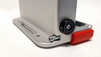
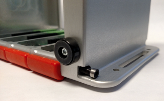
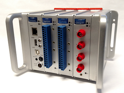
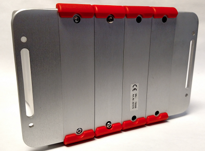
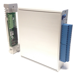
The controller and measurement modules of a Q.brixx system are each enclosed in their own aluminum shell along with an aluminum base. The base of each module attaches to the main body of each module using 2 x Torx T10 screws.
The bases are connected together, and the main body of each module interlocks together.
Each Q.brixx system also includes 2 x side pieces/handles (left side and right side).
The bases connect together using 2 x Allen screws (built into each base; the base for the controller is the exception).

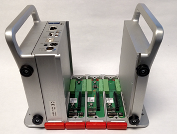
Assembling the Modules

Connect the handles and bases together. Start from the left side handle and move left to right. The right side handle will be secured last.
The controller is placed at the leftmost position (next to the left side handle). Therefore we need to connect the controller’s base to the left side handle. Secure the base to the left side handle using the 2 x Allen screws.
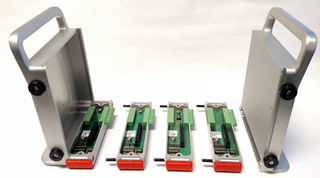
Connect all the bases together one by one, moving left to right.
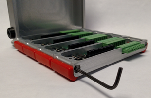
Secure the bases together using a 2.5 mm Allen wrench.
The right side handle attaches to the rightmost base and is secured using 2 x Allen screws.
Before securing the controller and measurement modules onto their bases, configure the DIP switches on the bases. Please refer to the configuration section below for more details.
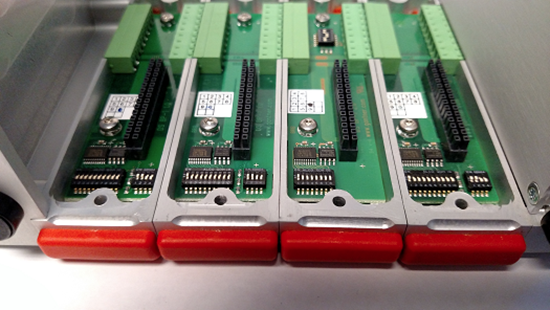
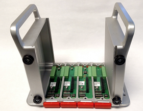
From left to right, secure the controller and measurement modules onto their bases.
All the modules interlock together.
Secure each module onto the base from the bottom. There are 2 x Torx T10 screws for each module.
Reverse the procedure to disassemble or replace any modules.

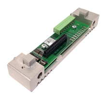
DIP Switch Configuration

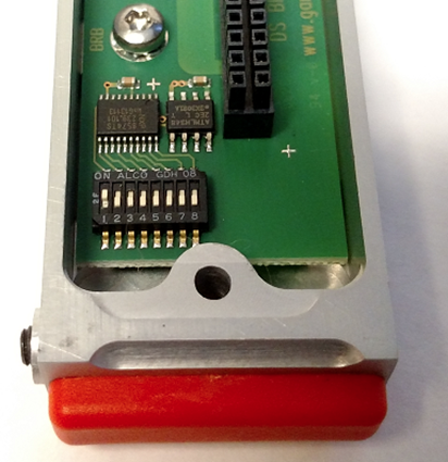
Unlike the Q.bloxx modules, where the address of the measurement modules is typically configured via software, the Q.brixx systems shipped from the factory have the address configured via the DIP switches. These DIP switches are located on the base of the module. Not only is the node address set using the switches, but terminating resistors and UART settings are also set using this method.

There are two versions of the Q.brixx base. Both versions work together on the same system. The difference between the versions is the location of the DIP switches.
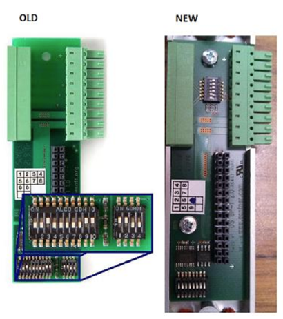
The “Older” version has 1 x 10-pin dip switch and 1 x 4-pin dip switch.
The 10-pin switch sets the address and/or terminating resistances.
PINs 1-6: Sets the address of the module (binary)
Terminating Resistance ON: PIN 9 and 10 Up
Terminating Resistance OFF: PIN 9 and 10 Down
The 4-pin switch is used to set the UART setting.
UART 1: PIN 1 and 2 Up (PIN 3 and 4 Down)
UART 2: PIN 3 and 4 Up (PIN 1 and 2 Down)
The “Newer” version has 1 x 8-pin dip switch and 1 x 6-pin dip switch.
The 8-pin switch is used to set the address (binary).
The 6-pin switch is used to set the UART and terminating resistance settings.
UART 1: PIN 1 and 2 Up (PIN 3 and 4 Down)
UART 2: PIN 3 and 4 Up (PIN 1 and 2 Down)

Bus Termination ON: PIN 5 and 6 Up
Bus Termination OFF: PIN 5 and 6 Down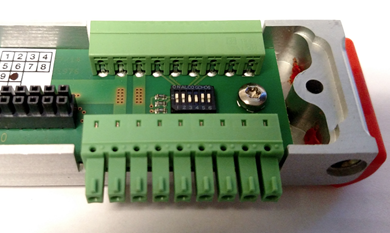

Binary Table for Address Setting:

Module Address	Switch Configuration
0 (reserved for the controller)	00000000
1	10000000
2	01000000
3	11000000
4	00100000
5	10100000
6	01100000
7	11100000
8	00010000
9	10010000
10	01010000
11	11010000
12	00110000
13	10110000
14	01110000
15	11110000
16	00001000

Key: 1 = UP , 0 = DOWN

Power Supply

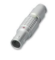
Like other Gantner systems, the Q.brixx system requires 10-30 VDC. This is delivered via the LEMO plug on the test controller's front.

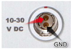
Each Q.brixx controller from the factory is shipped with an AC to DC adapter and power cable. Connect the adapter to the LEMO plug to provide power:

When the AC to DC adapter cannot be used, provide 10-30 VDC from a standard power supply; use LEMO connector part # FGJ.1B.302.CLLD42Z.

Sensor Connections

Standard Terminal Blocks

The Q.brixx system uses the same blue 10-pin terminal block on a standard Q.bloxx module. Sensor leads connect directly to these terminal blocks. If necessary, these terminal blocks are detachable from the main body of the module (for simpler installations and/or swapping sensor types).

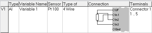
PIN assignment for a specific sensor type is displayed in ICP100 during the channel configuration process (more details in a section below). These connections are also available in the Q.brixx manual.

Example:

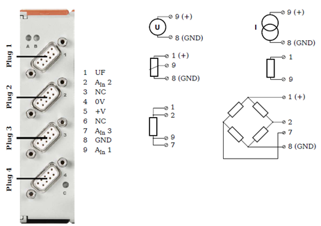
Special Connectors

The PIN connections for any special connections (DB9, BNC, mini TC, etc.) are available in the Q.brixx Manual.

Example:

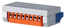
Special Terminal Blocks

The special terminal blocks used with Q.bloxx modules can also be used with Q.brixx modules. These terminal blocks are used for external cold junction compensation, bridge completion, and shunt resistance. Remove the blue terminal block the module is originally equipped with and replace it with the special one. Use the PIN assignment on the side of the terminal block to connect the sensor leads.

A101-CJC
A101-B4/120
A101-B4/350
A103-SR
A104-CJC
A107-CJC
A107-B4/120
A107-B4/350
A108-SR

Synchronizing Multiple Q.brixx Controllers

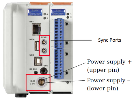
It is possible to synchronize multiple Q.brixx controllers together. In this setup, one controller is designated the master, and the rest are slaves. All controllers use the real-time clock of the master controller. Configuring the software settings for this feature will be explained in more detail in the section below.

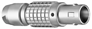
Each Q.brixx test controller (Q.gate and Q.station) has 2 x sync lines. Connect a sync cable from the master controller to the slave controller (1:1). The cable is a 2-wire twisted pair with LEMO connectors at both ends. The LEMO connector is part # FGG.00.302.CLAD30Z. The maximum length of all synchronization lines combined can be 1000 meters.

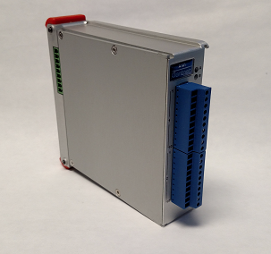
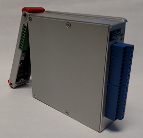
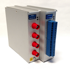
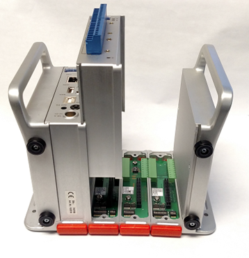
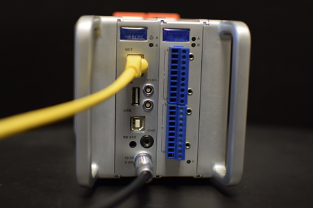
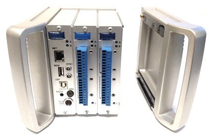
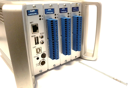
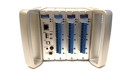
Q.brixx Controllers

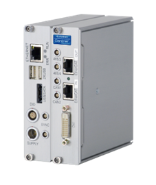
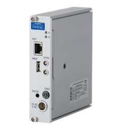
The standard Q.station, Q.gate-IP, and Q.gate-DP are all available in the Q.brixx housing. The Q.gate-DP and Q.station are fitted into double-wide housings to accommodate for the additional connections; the Q.gate-IP is in the standard single-wide housing.

Q.station:

Q.gate:

Connections

The Q.gate-DP has the same connections as the Q.gate-IP with adding 1 x Profibus-DP port. This DB9 is a Profibus standard connector with the following PIN configuration:

Connection	PIN
Vp = 5 Volts	6
TxD-P	3
TxD-N	8
GND	5

The Q.station has similar connections as the Q.gate-IP with the following additional interfaces:

Gigabit Ethernet (vs. 10/100 in Q.gate)
EtherCAT slave port (RJ45)
USB/SATA combo port
Digital Inputs (single LEMO connector Part # EGG.1B.308.CLL)

Connection	PIN
+5V Out	1
Digital Input 1	2
Digital Input 2	3
Digital Input 3	4
Digital Input 4	5
Digital Input 5	6
Digital Input 6	7
GND	8

DVI port: Used to transmit the built-in HMI screen.
2 x additional UARTs: 4 x UARTs total on a single Q.station, 2 connecting directly to the measurement modules via the base (the same method used with the Q.gate). The other 2 x UARTs are located on the front of the Q.station as a LEMO plug (part # EGG.00.302.CLL). The external connector is part # FGG.00.302.CLAD30Z.
CAN port: Used to connect to H and L of the CAN interface. This connection uses the same hardware as the UART and SYNC lines.

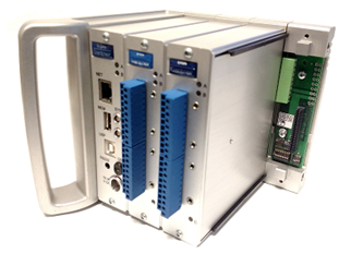
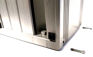
System Assembly (Q.brixx2)

The Q.brixx in the new housing design is similar to the original design. The electrical components of the modules, sensor terminations, and overall assembly method are the same. Projects configured on older Q.brixx will work in the new Q.brixx systems. This section will describe how to assemble a new Q.brixx system.

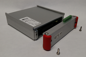
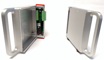
The individual modules of the new package are also contained in an aluminum housing that consists of a main body and a base.
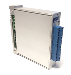
The complete Q.brixx system includes a left-side and right-side handle. Detach the right side handle to remove or add modules.
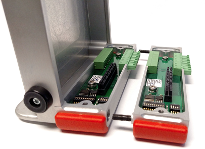
The base of the Q.brixx module contains the DIP switches for addressing and UART settings.
The bases connect together and are secured using a 7/64 hex key.
After securing the last base, connect the right side handle using the 2 x hex screws. Tighten the screws using a 3 mm hex key.
After securing the right side handle, the individual modules can be placed into their respective slots.
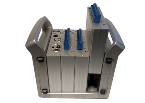
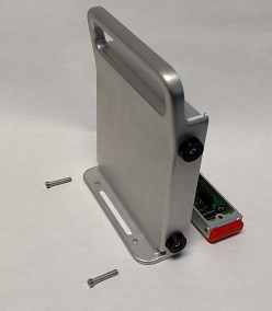
All the modules, including the controller, are secured to the base using 2 x long hex screws. Tighten the screws using a Torx T10 screwdriver.
After every module has been secured, the complete system is ready to be configured. If a module needs to be replaced or swapped, remove the 2 x long hex screws, slide the module out of the slot, and insert the new module.

PC Configuration

Two main settings must be configured on the PC to allow communications with a Gantner Instruments test controller.

Firewall – Provide exceptions for Gantner Instruments software tools
IP Address Configuration – If the Gantner system and PC are connected to the same network via a switch or router, the Gantner controller will obtain an IP address automatically using DHCP. If the Gantner controller and PC are connected without using a switch (direct Ethernet port to Ethernet port), the PC needs to have a static IP address on the same network as the Gantner controller.

Firewall

The test.commander software and other tools in the suite of Gantner software performs reads and writes to the hardware via Ethernet. The firewall on the PC (Windows or any 3rd party tools) must allow these tasks to occur.
To turn the Windows firewall off, open the Control Panel. Navigate to System and Security > Windows Firewall > Turn Windows Firewall on or off.
This will turn the firewall completely off.
To keep the Windows Firewall on, but provide exceptions to the Gantner software tools, open the Control Panel. Navigate to System and Security > Windows Firewall > Allow a program or feature through Windows Firewall. Within the list, select all Gantner tools or select the Allow another program button to add a program to the list. The list of Gantner tools:

- commander
- viewer
- ICP100
- ControllerUpdateTool
- SetupAssistant

IP Address

If the PC and Gantner system are connected to the same network, the PC and Gantner system will each obtain an IP address automatically (i.e., DHCP). By default, a Gantner test controller has DHCP enabled.
If the PC and Gantner system are connected together using an Ethernet cable, the PC requires a static IP address.
By default, a Gantner test controller ships with an IP address of 192.168.1.28. This IP can always be changed later, but for the initial connection, the PC needs to have a static IP address on the same network.
To change the static IP address of the PC, open the Control Panel. Navigate to Network and Internet > Network and Sharing Center > Change adapter settings.
Locate and double-click on the Local Area Connection. The Local Area Connection Properties window will appear:
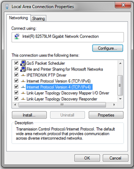
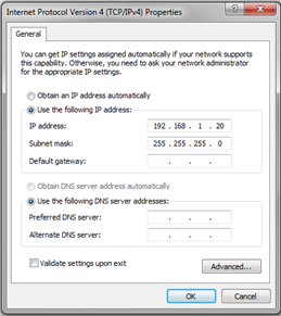
Under the Networking tab, double-click on Internet Protocol Version 4 (TCP/IPv4).
Within the TCP/IPv4 Properties window, give the PC a static IP address on the same network as the Gantner controller (i.e., 192.168.1.20) and a Subnet mask of 255.255.255.0

Starting test.commander

Applying the License & New Project

After downloading and installing test.commander, start the program by clicking on the test.commander icon.
Opening test.commander on a new PC will open in DEMO mode for the first time. Entering a test.commander license will convert the program into LICENSED mode. Enter the license information into the window provided:
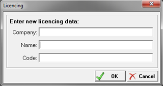
When the license is entered successfully, the program will change to licensed mode.
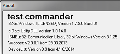
commander is now ready to create a new project.
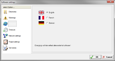
Language settings may need to be set. Extras > Settings, navigate to Language:
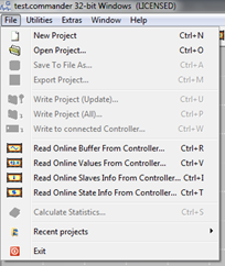
Select File > New Project.
Give the project a name.
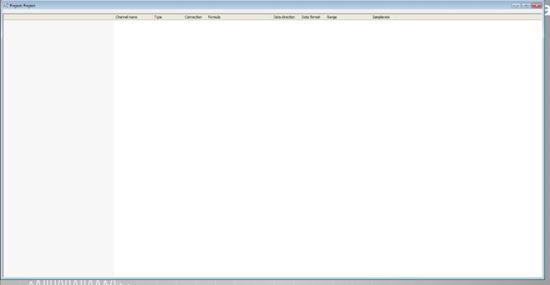
A blank project is now available.

Slave Setup

When a new system is being used, the first step is to assign a unique address to each measurement I/O module (skip this step if the address has been set using the DIP switches, typical for most Q.brixx systems). Two ways to assign an address to a measurement module are via the DIP switches mentioned in the previous assembly section or test.commander. This section will discuss how to set the address using the software method.
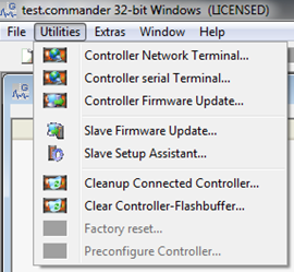
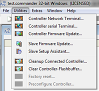
With a blank project open, select Utilities > Slave Setup Assistant:
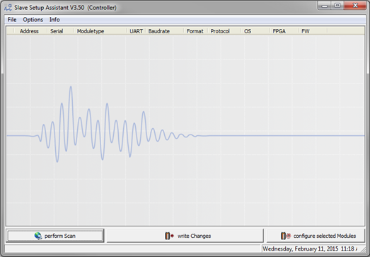
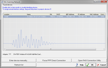
The Slave Setup Assistant window will appear. Click on the Perform Scan button to search for the attached controller.
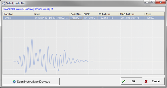
A separate window appears with all connected controllers. Highlight the controller for the current system and click OK.
The program will scan all UARTs (2 on a Q.gate and 4 on a Q.station/Q.pac) to search for all connected measurement modules. All modules that are found will be displayed in the Slave Setup Assistant window:
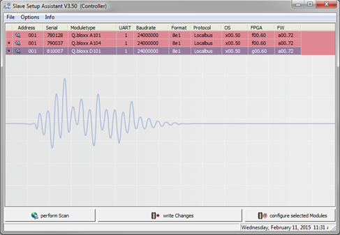
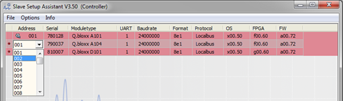
All measurement modules are shipped from the factory with a default address 1. To modify the address of any module, click in the cell under the Address column to change the address. Repeat the process for all modules.
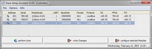
Click the Write Changes button to apply the new settings.

Firmware Updates

New Gantner hardware (controllers and measurement modules) is shipped from the factory with the latest version of the firmware. However, it is good practice to occasionally verify if the system has the most current firmware version. New firmware versions for controllers and measurement modules are included when a new version of test.commander is installed.
To check the firmware of a controller, select Utilities > Controller Firmware Update:
The program will search for all connected controllers, highlight the controller to connect to, and click the OK button.
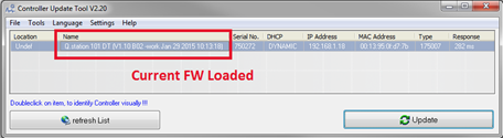
The Controller Update Tool appears; highlight the controller to update and click the Update button.
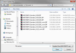
A window will appear with all FW versions available on the current PC. Select the FW to update the controller and click the Open button. An update is not required if the controller already has the most up-to-date version.
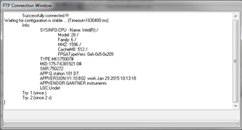
An FTP Connection Window will display the update process for a controller that requires an update. DO NOT remove power to the controller, and DO NOT disconnect the Ethernet cable during the update process.
To check the firmware version of a measurement module, select Utilities > Slave Firmware Update:
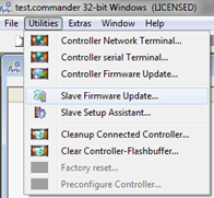
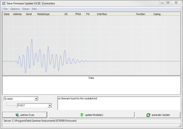
The Slave Firmware Update window appears; click the Perform Scan button.
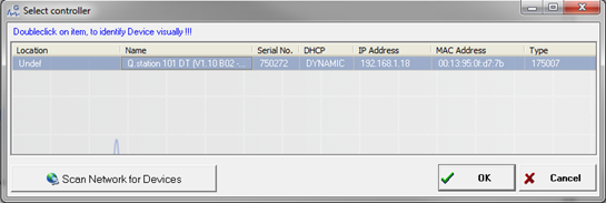
Highlight the controller to connect to and click the OK button.
The software scans all the modules. A green check mark represents an up-to-date module; a red mark means the module needs updating.
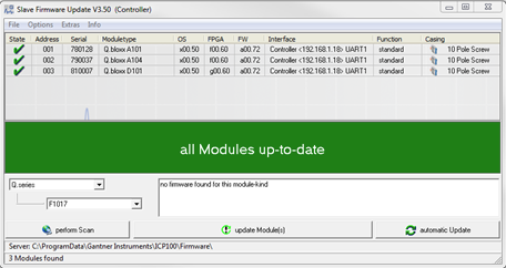
Clicking on the update Module(s) button will update all modules that require an update.

Connecting to the Hardware

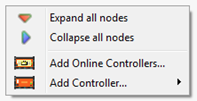
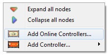
Within the blank project, right-click on the mouse and select Add Online Controllers.
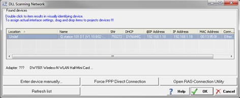
Select the controller to add to the project and click the OK button.
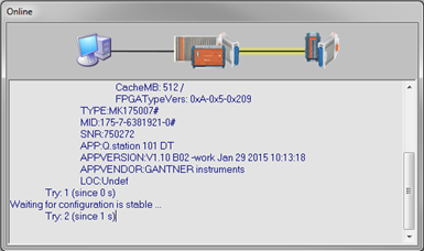
The Online window displays the reading process of the controller.
The following window appears at the end of the process; click OK.
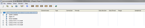
The controller and connected measurement modules are shown in the project.

Configuring a Controller

Controller’s Sample Rate (Q.station)

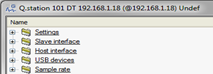
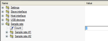
Double-click on the controller and navigate to the Sample rate.
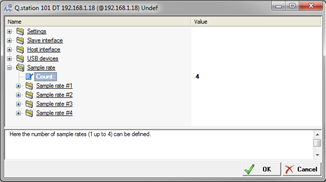
Having up to 4 x different sample rates in a Q.station is possible. Change the count value to add more sample rates.
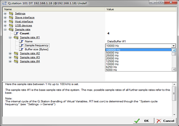
The name, sample frequency, and buffer size of each sample rate can be set. The sampling frequency can be set as high as 100 kHz. The 1st sample rate is the master rate. The 2nd, 3rd, and 4th sample rates can be the same or less as the 1st sample rate.
The buffer size of each sample rate can be modified. 200 MB of data buffer space can be split among the 4 x optional buffers.
The 1st sample rate receives its synchronization from the internal time clock. The 2nd, 3rd, or 4th sample rates can be synchronized from the internal time clock or one of the built-in digital inputs of a Q.station.

Controller’s Sample Rate (Q.gate)

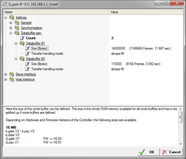
Double-click on the controller and navigate to Settings > Databuffer gen. Having 1 or 2 data buffers in a single Q.gate is possible. Both buffers use the same sample rate, but each buffer’s size can be modified. There is 16 MB available between all buffers.
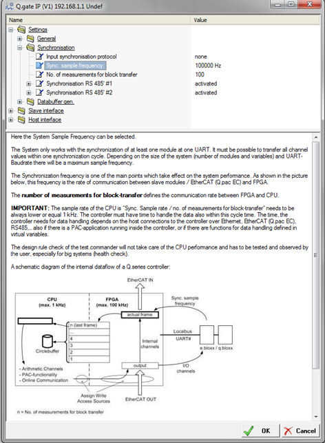
Navigate to Settings > Synchronization. The Sync. sample frequency can be modified:
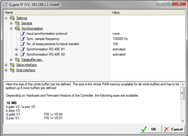
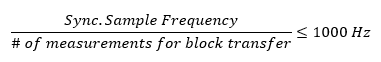
When the Sync. sample frequency is modified the No. of measurements for block transfer also needs to be modified. The number of measurements for block transfer defines the communication rate between the FPGA and CPU. The rule to follow is:

PAC Functionality Activation/Deactivation

There are many functional possibilities with the built-in PAC functionality of a Gantner test controller. To program the PAC functionality within a controller, we need the test.con software. To create and download a test.con project to a controller, the controller must be a “T” version. This must be specified at the time of purchase. This functionality must be activated.
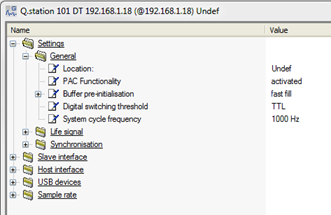
In a Q.station, navigate to Settings > General > PAC Functionality to activate or deactivate the feature.
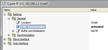
In a Q.gate, navigate to Settings > General > PAC Functionality to activate or deactivate the feature. When the PAC functionality is activated in the Q.gate, the data buffer can no longer be modified. The test.con program is saved to this memory.
Creating and downloading a test.con program into a Gantner test controller will be explained in further detail in our test.con quick start guide.

UART Configuration

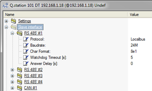
It is possible to configure the UARTs on a controller (2 x on Q.gate and 4 x on Q.station/Q.pac). These settings can be found by double-clicking on the controller and navigating to the Slave interface. The most important setting is the baud rate, which can be configured up to 24M. When the sample rate of the controller is reduced, it might be necessary to reduce the baud rate also.

Q.station:

Q.gate:

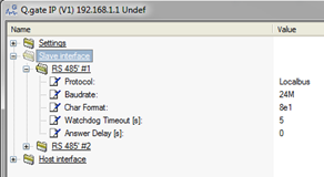
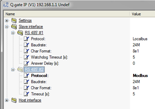
The 2nd UART of a Q.gate can be configured to use the Modbus protocol.

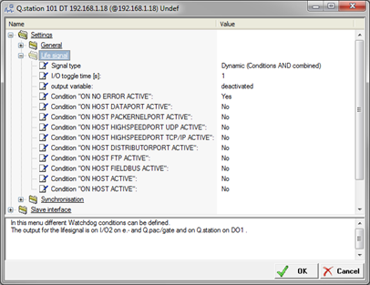
Life Signal (Q.station only)

The Q.station has built-in digital I/O, which can be used as life signals for various conditions.

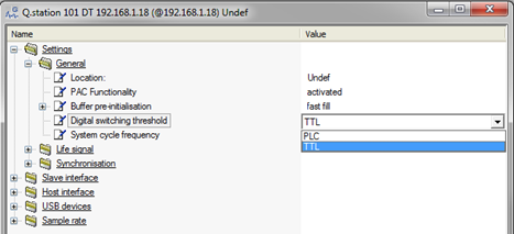
The switching threshold for the digital inputs can be set for TTL (5V) or PLC (10V) levels. Double-click on the Q.station and navigate to Settings > General > Digital switching threshold to modify this setting. This applies to all inputs.
The digital outputs on a Q.station can be used as a life signal based on preset conditions. The conditions can be switched on/off and combined as either AND/OR logic. To modify these settings, double-click on the Q.station and navigate to Settings > Life signal.

Interfaces (Q.station)

The Q.station has various communications interfaces for data transfer and data storage. These interfaces include CAN, EtherCAT, FTP, network drives, and E-mail. Configuring these interfaces can be found by double-clicking on the Q.station and navigating to the Host interface: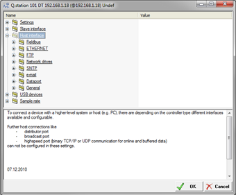

More information about utilizing and applying these interfaces can be found in separate start-up guides on the Gantner website.

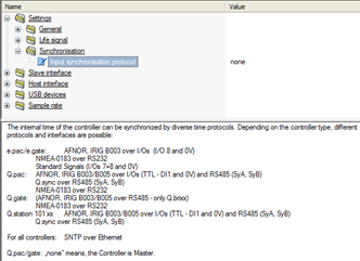
Synchronization Source

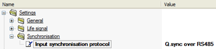
The controller can obtain its synchronization internally (built-in real-time clock) or externally (via SNTP, IRIG, GPS, AFNOR, or another Q.series controller). Double-click on the controller and navigate to Settings > Synchronization > Input Synchronization Protocol. If set to “none” the controller obtains its synch internally. Select a different method using the drop-down menu.

Double-click on the controller and navigate to Host Interface > SNTP > Client Settings to synchronize the controller via SNTP. Change the SNTP mode from Off to On. Enter the IP address of the location of the SNTP server. More information can be found in the “Synchronization via SNTP” guide on the Gantner website.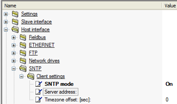

To synchronize the controller to another controller, set the Input Synchronization Protocol to Q.sync over RS485. For more details, please see the “Synchronization of Multiple Controllers” guide on the Gantner website.

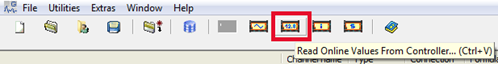
If the Input Synchronization Protocol is set to “none,” then we can perform a one-time synch of the controller’s internal clock with that of the attached PC.

Click on the Read Online Values From Controller button:
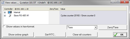
Click on the Set RTC button:
Ensure the radio button next to “Use local PC time” is selected. Click on the “Synchronize” button to apply the synch.
Time – date and time of the PC
Device – date and time of the controller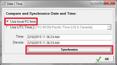

Channel Configuration

Real Variables

A real variable is configured in ICP100 (included with test.commander). Double-click on a module to open the module in ICP100. For this example, we will use an A101 module.

Double-click on the A101 module to open the module in ICP100:
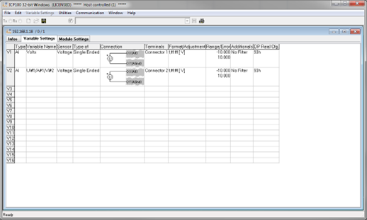
A new module will have the default settings loaded. For example, an A101 is a 2 x channel universal input module. There are 16 x slots available in each module. If 2 x real variables are used, 14 x remaining slots are available for arithmetics, signal conditioning, set points, and alarms.
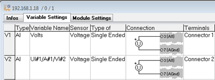
Type: This column selects the variable type (varies by module type). A real variable is an AI (Analog Input), AO (Analog Output), DI (Digital Input), or DO (Digital Output).
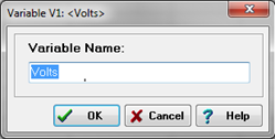
Variable Name: This column gives the variable a custom name. Each variable within a single controller needs to have a unique name.
Sensor: this column specifies the type of variable. The type of sensor to choose depends on the module being used. An A101 module is a universal input module. Therefore many possibilities are available:

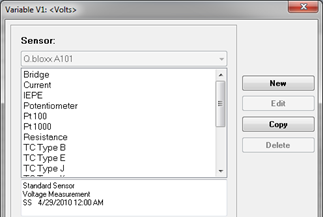
A modified version of any sensor can be created. This is necessary for sensors that have very precise calibration points. For example, a thermocouple can be factory calibrated.
Highlight the sensor to modify and click on the Copy button.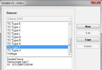

Give the new sensor a name.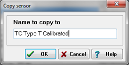

The new sensor will be added to the list. Highlight the new sensor and click on the Edit button.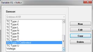

The sensor configuration window appears. This window provides more information about the pre-configured sensor. Click on the Lineariz. button.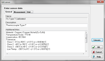

Highlight the unit to modify and click OK.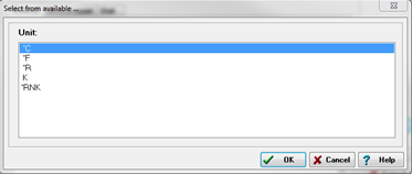

A sensor linearization table will appear. 300 individual measurement points can be used. Enter the measured value and displayed value for each point. The table can be exported and modified in a spreadsheet by clicking the Export button. A modified table can be imported by clicking on the Import button.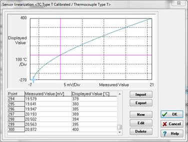
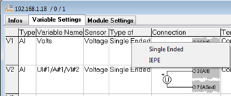
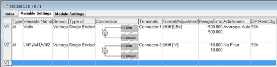
Type of: this column specifies the type of sensor (varies by module and by the sensor). For example, if a Voltage sensor is used on an A101, it can be configured as a single-ended or IEPE sensor.
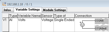
Connection: This column displays which PINs the sensor is physically connected to. The voltage sensor is wired across PINs 3 and 7 in the example below.
Terminals: this column specifies which connector to use on the measurement module. Each Gantner measurement module has 2 x connectors (a top and bottom). The top is connector 1, and the bottom is connector 2.
Format/Adjustment: this column is used to modify the way the variable is saved, including the units and format of the variable.

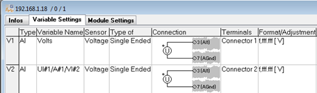
The variable can use the pre-defined unit selected based on the type of sensor used (for example, voltage sensor uses V or mV). However, the variable can be scaled to engineering units. Enter the units to use and click on the Scaling button.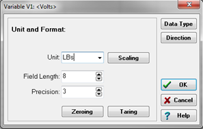

The variable can be scaled using either of the 2 x methods: point-point calibration or factory/offset. For this example, we will use the point-point calibration method.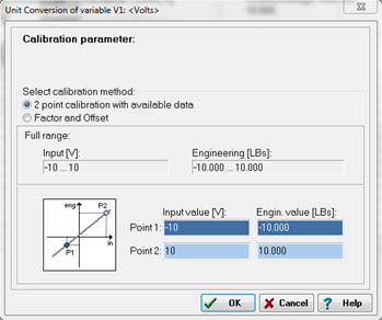

There are 2 x columns, the input value, and the Engin. value. There are 2 x points for each column, a low and a high end. The input value represents the physical characteristic that the sensor is measuring (i.e., Volts). The Engin. value represents the measured quantity we wish to save (i.e., LBs).

For this example, a ±10V input could represent ±500 LBs: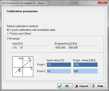

Click OK to confirm the setting changes.

Calibrating channels using live values: LINK
The Field Length sets the maximum number of digits the sensor will display.
The Precision sets the number of decimal places.
The Field Length needs to be at least 2+ the Precision.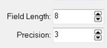

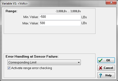
Zeroing and Taring are also configured in this section. A separate quick start guide that discusses how to apply the zero and tare feature can be found on the Gantner Instruments website: LINK
Range/Error: this column sets the minimum and maximum values to display. A value not within this range will result in an error/sensor failure. The behavior of sensor failure is also configured in this section. At failure, the sensor will display either:
1. Corresponding Limit
2. Stay at Last Value
3. User-selected Default Value
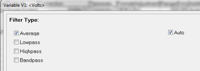
This error handling can be activated or deactivated.
Additionals: this column adds/removes/modifies any filters (average, lowpass, highpass, or bandpass).

Virtual Variables

Virtual Variables are variables that are composed of real variables and/or other virtual variables. These variables can be created inside the measurement module through arithmetic channels, signal conditioning channels or set points. They can also be created inside the controller under the virtual variables section.

Inside the Measurement Module

Double-click on the measurement module to open it in ICP100.
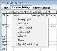
Find the next empty variable (V3 below) and click inside the Type column.
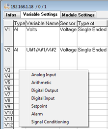
Select the type of virtual variable to create:

Arithmetic – uses standard math functions such as adding, subtracting, multiplying, and dividing. Also available are min, max, rms, and integration. Real and other virtual variables within the same measurement module can be used. Arithmetic variables are not computed at the same speed as the real variables.

Set point – the value of the set point can be obtained within the same module (source: internal) or from another measurement module (source: external). It can also be set to a constant.

Alarm – outputs a 0 if none of the conditions are met. Otherwise, it outputs a 1. Each alarm can have 4 x separate conditions combined as logical OR. The conditions to select from are shown below: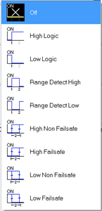

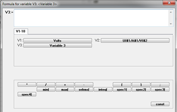
Signal Conditioning is similar to the arithmetic channels but cannot perform addition, subtraction, multiplication, and division. These variables are calculated at the same speed as the other real variables.
After selecting the variable type, the variable's specifics can be modified under the Additionals column. For example, the formula for an arithmetic variable can be created.
Make sure to save the configuration before closing ICP100.

Inside the Test Controller

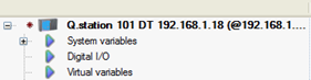
The Virtual Variables section is available under the test controller. Right-click on this section to add a new variable.
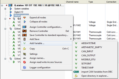
Select the type of virtual variable to add from the list shown above. It will be added to the virtual variables section.

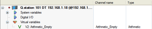
Arithmetic Empty is the most general version that can be used with the most flexibility. Standard math functions are available (adding, subtracting, multiplying, and dividing) along with a library of functions (i.e., average, min/max, comparison, PID). Any variable (real or virtual) within the same controller can be used within the arithmetic.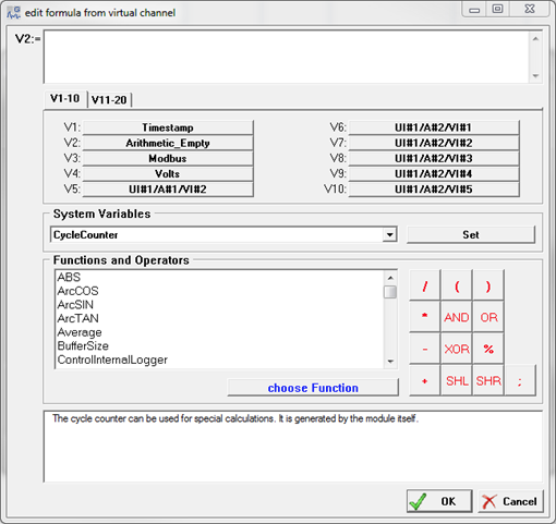

Modbus – slave devices can interface directly with a Q.station via the USB port. Connect an RS232 to RS485 converter (i.e., ISK103) between the Q.station and the slave. Configure the Modbus variable with the correct register settings/format.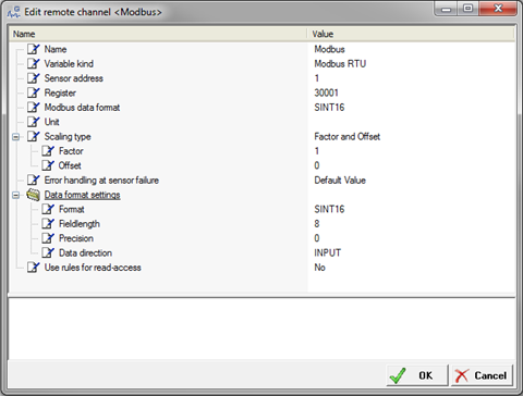

CAN Input – reading and writing CAN data with the Q.station is possible. We set up the CAN inputs under the virtual variables section. Double-click on the CAN Input to modify the CAN ID, byte order, format, start bit, and bit length. If a CAN database file is available, the pre-defined variables can be selected from this file; click the CAN DB button to navigate to the file.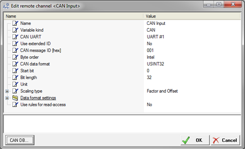

Set point – a standard set point can be created here. The format of the variable is also available.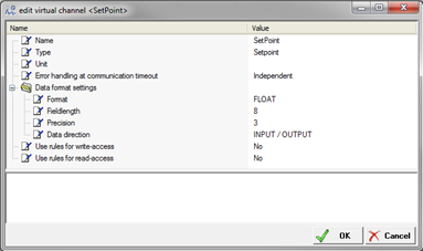

Naming Variables in Batches

Naming a variable (real or virtual) is as easy as typing in the desired name. This method is perfect for small to medium-sized projects. When large projects are being created, it might be necessary to name variables in batches, especially for identical sensors that are incrementing (Volts 1, Volts 2, …, Volts 20, etc.).

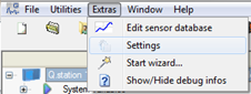
In test.commander, select Extras > Settings.
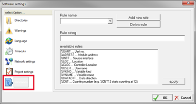
Select the Variable Names option.
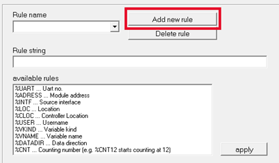
Click on the Add new rule button.
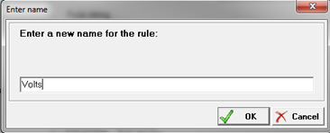
Give the rule a name.
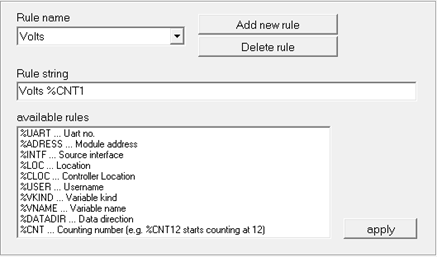
Define the variable’s format in the Rule string section.
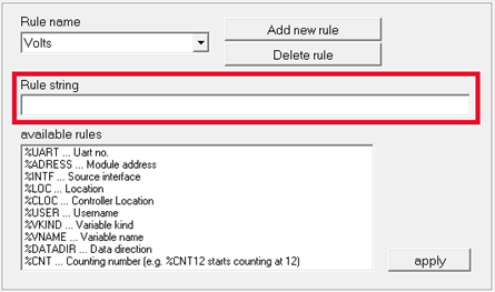
Use the pre-set rules to create the custom string. For example:
Click the OK button to save the rule.
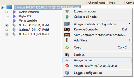
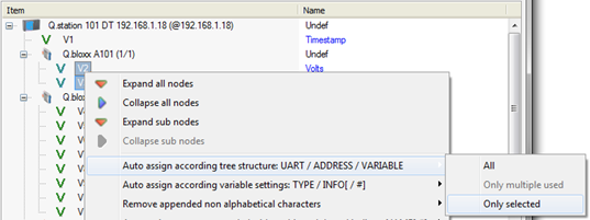
Right-click on the controller and select Assign names.
Highlight the Variables to rename and right-click on the selected variables.
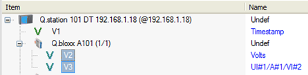
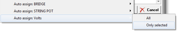
It is possible to auto-assign names using the pre-set methods (UART/ADDRESS/VARIABLE or TYPE/INFO) or using one of the rules we created.
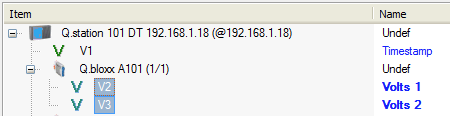
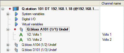
Click the OK button to apply the new settings. The variables have been renamed in the project; make sure to update the project to the controller to finalize the process.

Data Logger Configuration – Q.station

This section describes how to configure the Q.station’s data logger. Please use this guide and the Q.station manual (pages 59-85) for complete information.

Rules

The data logger built into the Q.station is very flexible, but there are some rules to follow to create a functional system.

It is possible to configure up to 4 x separate data buffers. Each data buffer can have a unique sample rate. The 1st data buffer is the master rate; the 2nd, 3rd, and 4th buffers can be configured to have the same sample rate or smaller (can’t be greater than the 1st)

Configuring up to 4 x separate UARTs on a single Q.station is possible. A single UART can be configured for 1 x data buffer (i.e., 1 x sample rate). Modules/channels under a single UART can’t be split into more than 1 x data buffer.

Incorrect: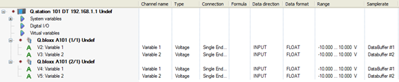

Correct: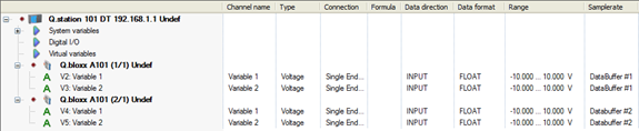
The 1st data buffer is the basic sample rate of the entire Q.station. Therefore it must obtain its synchronization source internally. Data buffers 2 to 4 can obtain its synchronization internally or externally (i.e., angular synchronization).
Creating up to 20 x separate data loggers within a single Q.station is possible.
A single data logger can obtain data (i.e., channels/variables) from 1 x data buffer.
The logging rate of a data logger can be the same or less than the data buffer it is assigned to.

Sample Rate Assignment

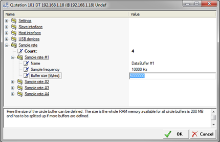
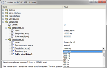
Configure the number of data buffers to create. Double-click on the Q.station and navigate to Sample rate > Count. Enter the number of sample rates (1 to 4).
Give each sample rate a name, sample frequency, and buffer size.
The name is used to distinguish one sample rate from the rest.
The sampling frequency is the update rate of the buffer. This can be configured up to 100 kHz.
The buffer defines how large the buffer is. There is 200 MB available that must be shared between all buffers (up to 4).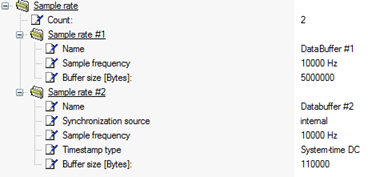
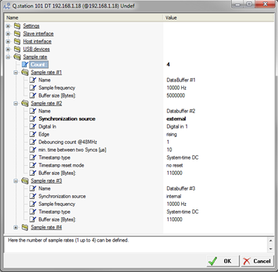
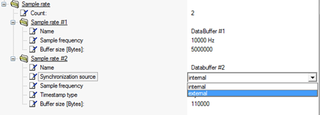
The rules section mentions that the 1st sample rate obtains internal synchronization. The synchronization source for sample rates 2 to 4 can be obtained internally or externally. To set externally, change the synchronization source:
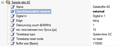
Additional settings become available when set to external. For more details, please see pages 60-61 and 85 of the Q.station manual.

Apply Sample Rate to Measurement Modules

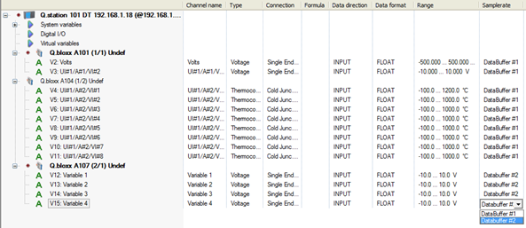
There is a Sample rate column in the test.commander project. Using this column, apply the desired sample rate for each channel. Remember that variables/channels on a UART must share the same sample rate.

The measurement modules in the test.commander project displays the UART and address for which they are configured.

Example:

Q.bloxx A101 (1/1) = Q.bloxx A101 (UART 1/Address 1)

Q.bloxx A104 (1/2) = Q.bloxx A101 (UART 1/Address 2)

Q.bloxx A107 (2/1) = Q.bloxx A101 (UART 2/Address 1)

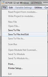
Accessing Logger Configuration

The preliminary settings are now configured. Highlight the Q.station and click the Logger configuration button.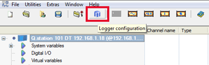

Complete details on configuring the Q.station data logger can be found in the separate guide.

Data files saved using the Q.station logger are saved in .DAT file format. These are universal data bin files (UDBF), a binary file that contains a header section followed by raw binary data. These .DAT files can be opened using test.viewer for post-processing.

Project Verification

System Check

After configuring the controller, configuring all the channels/variables, and setting the data logger configuration before updating the project to the controller, it is beneficial to analyze the project's feasibility.

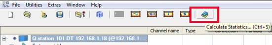
Select the Calculate Statistics button.

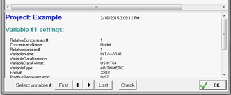
Select the Check button.

The Design Rule Check window will appear. The background color displays the feasibility:

White = Will work

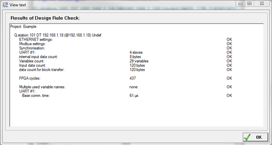
Red = Will not work

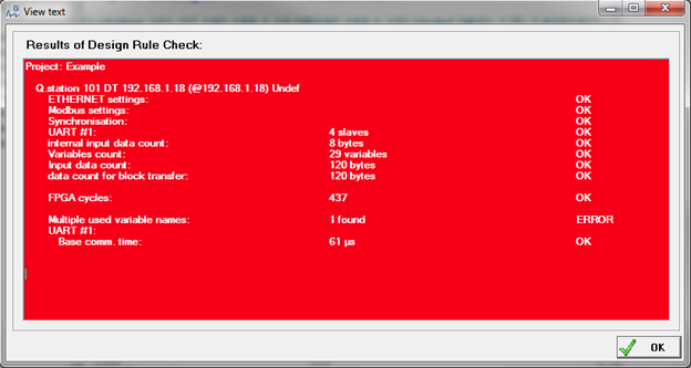
Yellow = Might work

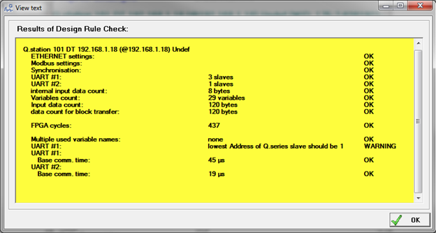
The cause of the issue is shown next to the warning/error. Change the appropriate settings before proceeding (sample rate, UART baud rate, number of channels, and variable names are just a few of the most common issues). After all, settings have been correctly configured, the project can be updated to the controller: File > Write Project (Update).

Viewing & Saving Live Data

After the project has been verified and updated to the controller, it is possible to view the live data stream. This is performed using the built-in tool called test.viewer.

Select the Read Online Values From Controller button: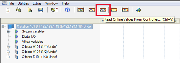

The View Values window appears. Use this page to verify if all appropriate sensors are connected. Check for any data dropouts (if any error counters are accruing).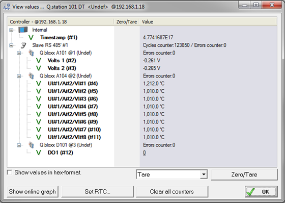

Click on the Show online graph button to open test.viewer.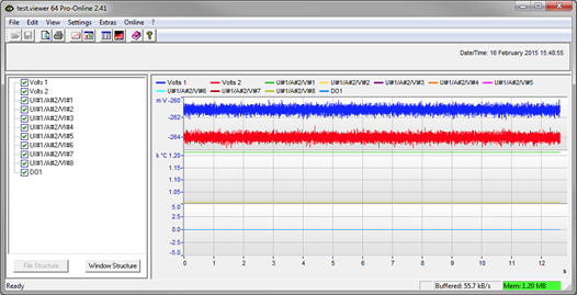

The data can be analyzed using test.viewer. To save the data, select Online > Stop Live Stream.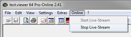

Select File > Save As.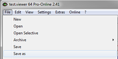

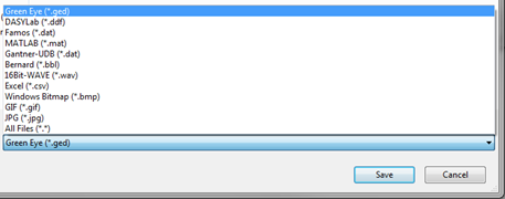
Select a name for the file and the format in which to save it.

Exporting Projects

The test.commander project is saved in the projects folder within the Gantner directory of the PC. When the project is updated to the controller, it is also saved inside the controller.

To modify the project on a different PC:

Install test.commander and apply the license on the new PC.
Connect the hardware to the new PC using a standard Ethernet cable.
Open test.commander and create a new/blank project.
Right-click in the workspace and select Add Online Controllers.
The project inside the controller is now available on the new PC.

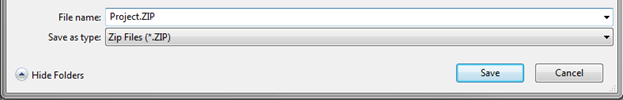
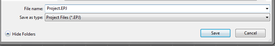
It is also possible to export a project that is open in test.commander to a ZIP file. This ZIP file can then be transferred to a different PC using an external storage device (i.e., USB thumb drive) or E-mail.

File > Export Project
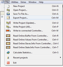
Give the ZIP file a name and click Save.

Q.brixx Classic - Quick Start Guide

The complete start-up guide for assembling and configuring the Gantner Instruments Q.brixx measurement and test automation system

Table of Contents

System Preparation

Introduction

Software Requirements

Software Downloads

PC Requirements

Accessories

System Assembly (Q.brixx 1)

Description

Assembling the Modules

DIP Switch Configuration

Power Supply

Sensor Connections

Standard Terminal Blocks

Special Connectors

Special Terminal Blocks

Synchronizing Multiple Q.brixx Controllers

Q.brixx Controllers

Connections

System Assembly (Q.brixx2)

PC Configuration

Firewall

IP Address

Starting test.commander

Applying the License & New Project

Slave Setup

Firmware Updates

Connecting to the Hardware

Configuring a Controller

Controller’s Sample Rate (Q.station)

Controller’s Sample Rate (Q.gate)

PAC Functionality Activation/Deactivation

UART Configuration

Life Signal (Q.station only)

Interfaces (Q.station)

Synchronization Source

Channel Configuration

Real Variables

Virtual Variables

Naming Variables in Batches

Data Logger Configuration – Q.station

Rules

Sample Rate Assignment

Apply Sample Rate to Measurement Modules

Accessing Logger Configuration

Project Verification

System Check

Viewing & Saving Live Data

Exporting Projects