How to perform FFT and spectral analysis

Using the FFT processor and evaluators

 

Introduction

FFT (Fast Fourier Transform) analysis and visualization are possible with the Q.series X DAQ system. A controller can be configured to generate and analyze FFTs in real-time, independent of a computer. The GI.bench software includes FFT charts to o visualize the frequency spectrum of your signal(s).

This quick start guide will provide an introduction to the FFT capabilities and how to begin configuring a system.

Virtual variables for FFT functions

The controller can be configured with up to 512 virtual variables. One type of virtual variable is the arithmetic variable, which can be customized with various functions and variables.

GI.bench

Virtual variables for generating the FFT spectra and performing evaluations can be done quickly through the controller settings section or manually by creating the arithmetic virtual variables with the corresponding functions.

If creating manually, proceed here to create variables, here to generate spectrum, and here to create evaluators

1. Double-click the controller to open the Controller Settings

2. Navigate to the Functions section, and enter an FFT processor count for the number of FFT processors to be created

3. Select FFT #1 below the Functions section.

a. Select the data stream and the desired FFT input variable 

b. Enter the desired FFT settings e.g. size, window type. Make sure to have enough points to the window to increase spectral resolution.

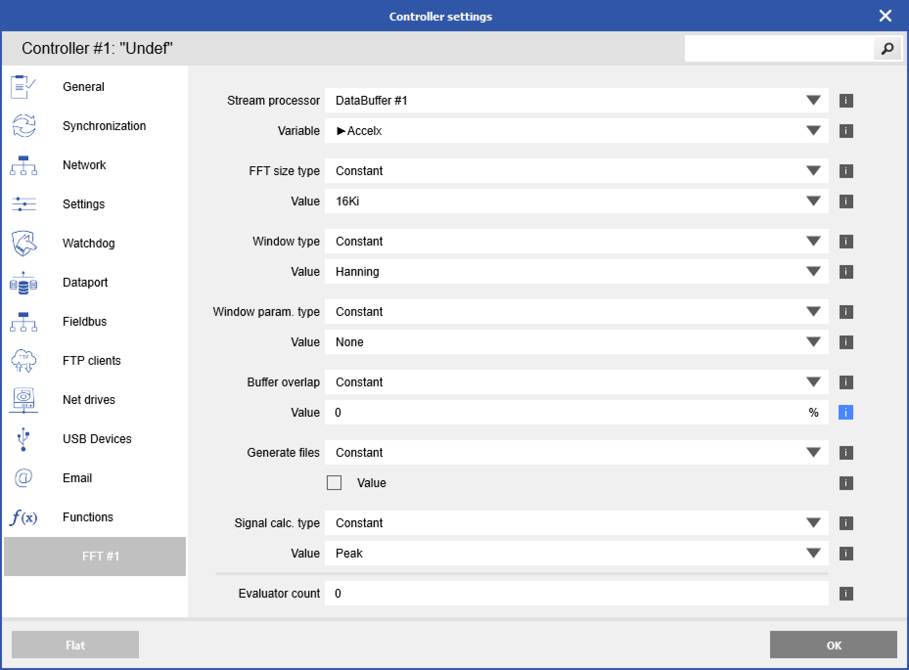
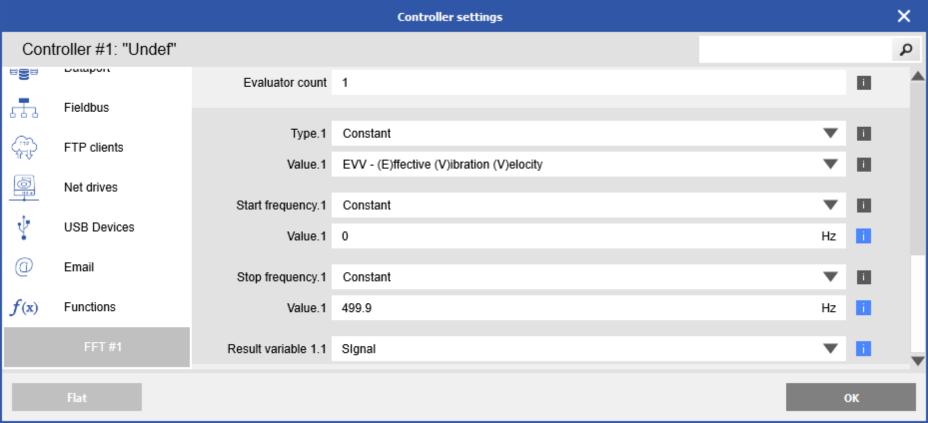
4. Enter an Evaluator count to add a number of evaluators for FFT analysis

a. Select the type of evaluation under the type 1 value e.g. min, max, RMS,  vibration displacement, vibration velocity. If the accel channel was already scaled to m/s^2, the result of EVV calculation would give a value with units of m/s.

b. Enter the start and stop frequencies (constant or by a variable)

c. Select the variable where the results will go (e.g. a virtual setpoint variable)

5. When complete click OK and write updates to the controller.

Manual Method

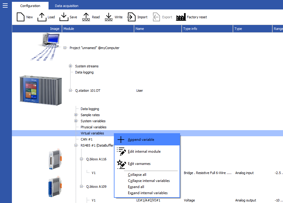
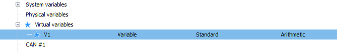
To create a new variable right-click on Virtual variables under the Q.station and click Append Variable. It will ask how many variables you want to create.

Double-click on the newly created arithmetic channel to open the settings window.

The menu can be viewed in a flat or structured layout. Click on the Formula tab and go to the Formula text section to make changes. Select the function from the Functions drop-down list. Click the [i] icon to learn how to configure that function. Click Set at Cursor to enter the function at the current cursor location in the Formula text box.

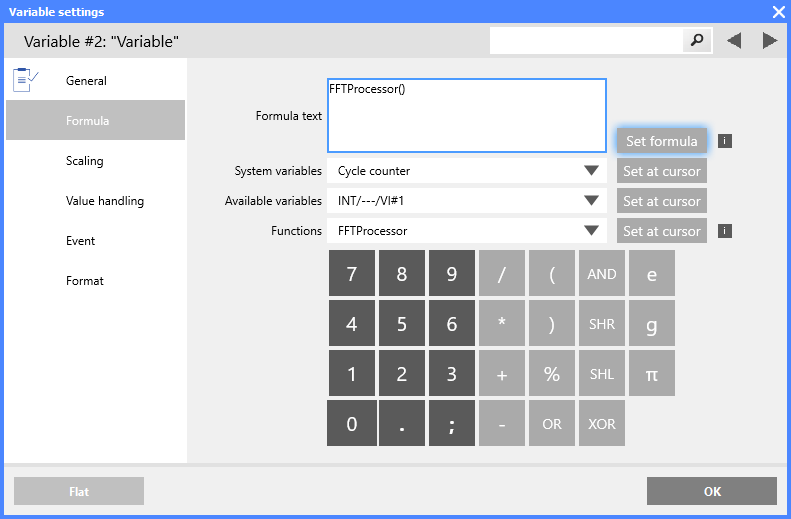
Other variable settings can be adjusted by going to the other categories e.g. scaling and format.

---

test.commander

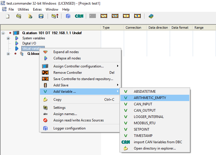
To create a new variable right-click on Virtual variables under the Q.station and go to Add Variable > Arithmetic Empty

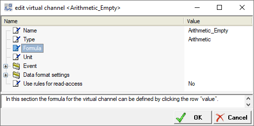
Double-click on the newly created arithmetic channel to open the settings window. Click on the Formula text to open the formula configuration window.

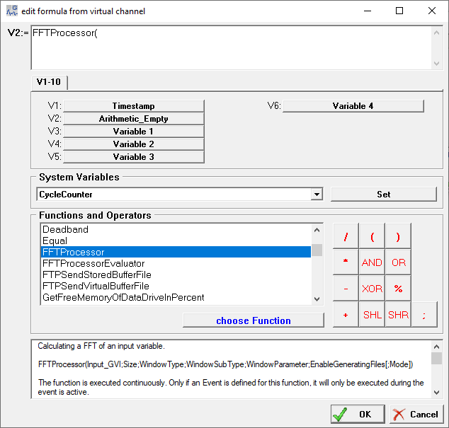
Select the desired function from the list below. Clicking on the function will provide instructions on what it does and how to set it up. Double-click the function to enter it into the formula. Select the appropriate variables/values depending on the function.

---

FFT Processor & Evaluator Details

Amplitude spectrum can be calculated directly on the controller and results like minimum, maximum, or velocity can be written to a virtual variable as a channel. Results can be used for alarm generation and component stop via digit output for instance.
The configuration should be done on the following principle:

• Definition of the evaluation parameters as setpoint
• Configuration of the FFTProcessor (spectrum calculation)
• Configuration of the FFTEvaluator (spectrum evaluation)

Generate FFT spectrum

FFTProcessor
FFTProcessor(VariableIndex;Size;WindowType;WindowSubType;WindowParameter;EnableGeneratingFiles[;Mode;TimeDomainBufferOverlappingPercentage])

Definition of parameters:
VaraibleIndex: This is the index of the input variable placed in at least one DataBuffer. Timestamp variable can NOT be used. Range: 0 … variables count – 1

Size: N_samples, number of points to be calculated.
IMPORTANT: It must be a power of 2. Note that each point requires 52 bytes of internal memory for calculation. Range: 4 – 1048576.

WindowType: define which window form to use:
0: Blackman
1: BlackmanNuttal
2: BlackmanHarris
3: BartlettHanning
4: Exponential or Poisson
5: FlatTop
6: Gaussian
7: Hamming
8: Hanning
9: Kaiser
10: Lanczos
11: Nuttal
12: PowerOfCosine
13: Rectangular or None
14: Triangular or Bartlett
15: Welch

WindowSubType, WindowParameter, EnableGeneratingFiles: enter a value of 0

Example:
FFTProcessor (80;V23;8;0;0;0)
80: V81 is the accelerometer analog input
V23: virtual variable setpoint to change the parameter of the size
8: Hanning window type

Evaluation of FFT Spectrum

The FFTProcessorEvaluator function is used to perform analysis on the FFT Spectrum calculated using the FFTProcessor function. The type of analysis is dependent on the function’s parameters.

FFTProcessorEvaluator

FFTProcessorEvaluator(FFTProcessor;Function;StartFrequency;StopFrequency;Result1VariableIndex;Result2VariableIndex)

Description of parameters:
FFTProcessorReferenceVariable: This is the variable of the FFTProcessor to be used.

Range: V1 … Vn

Function: Type of evaluation on the FFT spectrum signal
0: FFT Error States
1: Minimum
2: Maximum
3: Integral
4: RMS (Root mean square)
5: SINAD* (Signal-to-interface ratio, including noise and distortion)
6: ENOB* (Effective number of bits)
7: SNR* (Signal-to-noise ratio)
8: THD* (Total harmonic distortion)
9: SFDR* (Spurious free dynamic range)
10: EVV (Effective vibration velocity)
11: EVD (Effective vibration displacement)

*Best with Hanning-Window
Take care that single-sine-tone signal source has better quality than you expect as result
Signal level should be in full range of used input

Start/Stop Frequency: This depends on your application and the type of evaluation.

Start frequency: frequency to start the evaluation
Range: 0 to (Nyquist frequency – bin frequency); < stop frequency

Stop frequency: frequency to end evaluation
Range: 0 to (Nyquist frequency – bin frequency); > start frequency

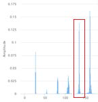
Example: If evaluating the max of this peak, you would enter a start and stop frequency near this range

Result1VariableIndex;Result2VariableIndex: resultant values depending on function type

---

Effective Vibration Velocity Example

In this example using a 104mV/g IEPE sensor and calculating the effective vibration velocity (EVV).

1. Configure accelerometer analog input channel. Converting driectly from g to m/S^2 with factory 9.81
   
2. Configure FFT Processor in Controller Settings window. Use a Hanning or Flat Top window for example. Make sure there is enough points to the window to increase spectral resolution.
   
3. Add FFT Evaluator with type of (E)ffective (V)ibration (V)elocity
   
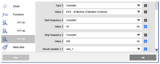
4. The result with be in m/s. You can multiply by 1000 in an arithmetic virtual variable to get a value in units of mm/s.
   
   
   
5. Calculated value matches shaker checker