Table of Contents
Configuration (test.commander)
- Configuring a Controller
- Channel Configuration
- Data Logger Configuration – Q.station
- Project Verification
- Viewing & Saving Live Data
- Exporting Projects
- Index
Accessories Required
- Ethernet cable (CAT5e or better)
- Electrical cable (18-22 AWG)
- Power adapter (10-30 VDC)
System Assembly
Assembling the Modules
After unpacking the hardware (controllers and measurement modules), one of the first things to determine is where to install the system. All the units are DIN rail mountable (35 mm DIN rail according to DIN EIN 60715),
Q.bloxx modules are mounted on a DIN rail using the Q.socket, which is provided with the shipment.
The Q.station 101 or Q.monixx is equipped with the following built-in mounting clamp: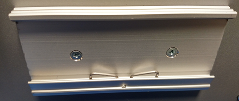
Electrical wiring
A system consisting of a Q.station 101 or Q.monixx controller and Q.bloxx modules must be electrically connected using wire (typically 18–22 AWG). The controller is mounted directly onto the DIN rail. Using the same method described above, mount and connect the Q.bloxx modules adjacent to the controller.
For example, to connect the UART interface between a Q.station and the Q.bloxx modules, make the following wiring connections:
|
UART |
Q.station 101 Connection |
Q.bloxx Connection |
|
1 |
A1 |
1A |
|
B1 |
1B |
|
|
2 |
A2 |
1A |
|
B2 |
1B |
|
|
3 |
A3 |
1A |
|
B3 |
1B |
|
|
4 |
A4 |
1A |
|
B4 |
1B |
|
UART |
Q.monixx |
Q.bloxx Connection |
|
1 |
RS485 A |
1A |
|
RS485 B |
1B |
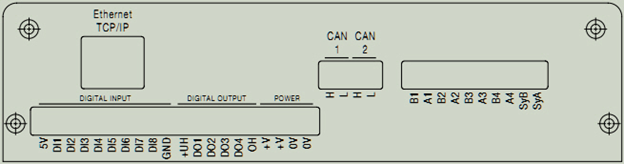
Q.station 101 (bottom view):
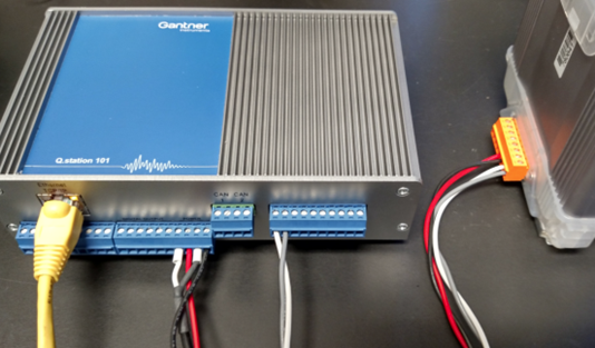
Example (Q.station connected to Q.bloxx modules via UART1):
Q.monixx to Q.bloxx classic
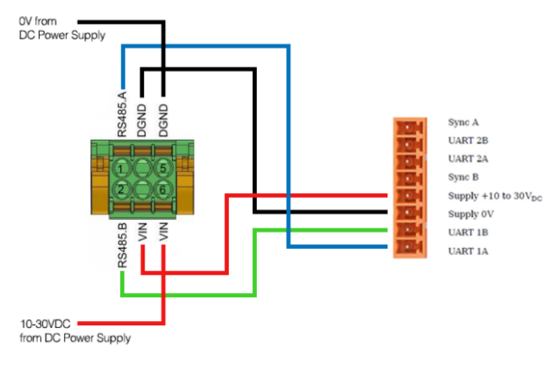 The Q.station X can connect to classic modules using the extension socket right or UART/power right. VIN to Supply+, GND to Supply 0V, A1 to UART 1A, and B1 to UART 1B.
Configuring the DIP Switches
- Module Address
Each Q.bloxx module on a given UART needs to have a unique address. In most applications, the first module on a UART starts at address 1. The address of a module can be set via the DIP switches on the Q.socket or using the Slave Setup Assistant tool in test.commander. Setting the address using the DIP switches is optional for most applications but is required when the hot swap feature is activated.
The address on the Q.socket is set in binary form using the first 6 x switches. An address of 0 corresponds to no configuration; therefore, the module obtains its address via software using the Slave Setup Assistant tool. All Q.bloxx modules shipped from the factory have a default address of 1 (software configured).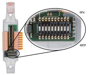
A Q.bloxx module’s address can be 1 to 32:
OFF = Down, ON = Up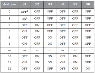
Note: The Q.gate does not require an address; therefore, all switches should be down. - Hot Swap Feature
The module configuration is loaded onto the Q.socket (EPROM) when the hot swap feature is activated. With this activated, a defective module can be replaced by simply removing it from the socket and replacing it with the same module type. The new module will obtain the configuration from the base.
The hot swap feature is activated whenever the module’s address is set via the base.
To set the module’s address via the base and deactivate the hot swap feature, ensure DIP switch 8 is ON. - Terminating Resistances
The terminating resistances must be activated on the last base of each UART. This is done to prevent reflections on the line that could lead to disturbances or loss of data transmission. The Q.socket that holds the Q.gate does not need the terminating resistances because this module contains its own resistances internally.
Push DIP switches 9 and 10 UP to activate the terminating resistances.
Connecting Sensors
Each Q.bloxx module is different (connects to different types of sensors and different channel counts). PIN layout and sensor connections for each module can be found in the Q.bloxx manual (page 44-91): LINK
Distributed Layout
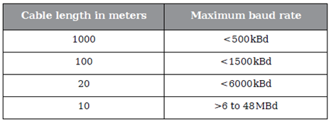
In some applications where the measurement modules are located in different locations than the test controller, a certain length of electrical wire is used to connect the system. This overall cable length on a single UART affects the data transmission; therefore, the maximum baud rate for that UART needs to be reduced.
Use the table below as a guide to determine the relationship between cable length and maximum baud rate. We will discuss how to configure the baud rate in the software section. Controllers and measurement modules shipped from the factory use a default baud rate of 24 MBd. The Q.station X can support up to 48MBaud.
PC Connection
- With the modules mounted onto the DIN rail and connections between the controller and measurement modules secured, the complete system can be connected to the PC. Connect an Ethernet cable from the Ethernet port of the PC to the Ethernet port of the Gantner Instruments test controller.
The test controller can connect to a network via a switch as a second option.
PC Configuration
Two main settings need to be configured on the PC to allow communications with a Gantner Instruments test controller.
- Firewall – Provide exceptions for Gantner Instruments software tools
- IP Address Configuration – If the Gantner system and PC are connected to the same network via a switch or router, the Gantner controller will obtain an IP address automatically using DHCP. If the Gantner controller and PC are connected without using a switch (direct Ethernet port to Ethernet port), the PC needs to have a static IP address on the same network as the Gantner controller.
Firewall
See article: https://knowledge.gantner-instruments.com/firewall-and-network-settings-guideIP Address
- If the PC and Gantner system are connected to the same network, the PC and Gantner system will each obtain an IP address automatically (i.e. DHCP). By default, a Gantner test controller has DHCP enabled.
- If the PC and Gantner system are connected together using an Ethernet cable, the PC requires a static IP address.
- By default, a Gantner test controller ships with an IP address of 192.168.1.28. This IP can always be changed later, but for initial connection, the PC needs to have a static IP address on the same network.
- To change the static IP address of the PC, open the Control Panel. Navigate to Network and Internet > Network and Sharing Center > Change adapter settings.
- Locate and double-click on the Local Area Connection. The Local Area Connection Properties window will appear:
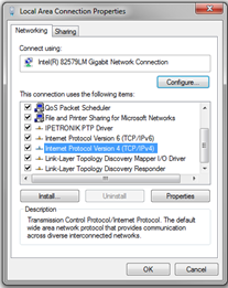
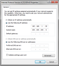
- Under the Networking tab, double-click on Internet Protocol Version 4 (TCP/IPv4).
- Within the TCP/IPv4 Properties window, give the PC a static IP address on the same network as the Gantner controller (i.e. 192.168.1.20) and a Subnet mask of 255.255.255.0
Configuration (GI.bench)
GI.bench can only be used with Q.station or Q.monixx controllers
Applying the License & New Project
- After download and installing GI.bench, start the program by clicking on the GI.bench icon.
- Opening GI.bench on a new PC for the first time will show the license options.
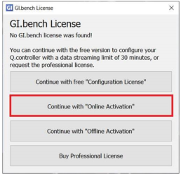
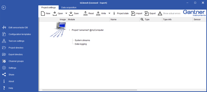
https://knowledge.gantner-instruments.com/how-to-license-activate-gi.bench-software - GI.bench will show a blank project
Slave Setup
- When a new system is being used, the first step is to assign a unique address to each measurement I/O module. There are two ways to assign an address to a measurement module: via the DIP switches mentioned in the previous assembly section or using test.commander. In this section, we will discuss how to set the address using the software method.
- With a blank project open, select Utilities > Slave Setup Assistant:

- The Slave Setup Assistant window will appear. Click on the perform Scan button to search for the attached controller.

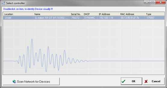
- A separate window appears with all connected controllers. Highlight the controller for the current system and click OK.

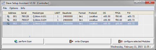
- The program will scan all UARTs (2 on a Q.gate and 4 on a Q.station/Q.pac) to search for all connected measurement modules. All modules that are found will be displayed in the Slave Setup Assistant window:

- All measurement modules are shipped from the factory with a default address of 1. To modify the address of any module, click in the cell under the Address column to change the address. Repeat the process for all modules.

- Click the write Changes button to apply the new settings.
Firmware Updates
- New Gantner hardware (controllers and measurement modules) are shipped from the factory with the most up to date version of the firmware loaded. However, it is good practice to verify if the system has the most current firmware version from time to time. New firmware versions for measurement modules are included when a new version of GI.bench is installed. Controllers are updated with GI.bench, modules currently with test.commander.
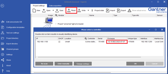
- To check the firmware of a controller, select Read in the Project Settings tab
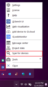
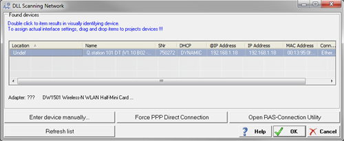
- To search for and install new Q.station firmware, right-click GI.icon in system tray and select Scan for Devices
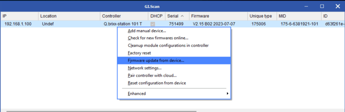
- In the GI.scan window, you can check for new firmware zip files online or initiate the firmware update
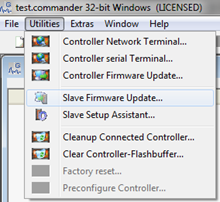
- To check the firmware version of a measurement module, in test.commander select Utilities > Slave Firmware Update:
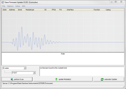
- The Slave Firmware Update window appears, click the perform Scan button.
- Highlight the controller to connect to and click the OK button.

- The software scans all the modules. A green check mark represents an up to date module and a red mark means the module needs to be updated.

- Clicking on the update Module(s) button will update all modules that require an update.
Connecting to the Hardware
- Within the blank project, click Read, select the controller and click OK
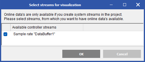
- A popup asking if you want to automatically create a PC systemstream from the already configured variables. Click OK or cancel
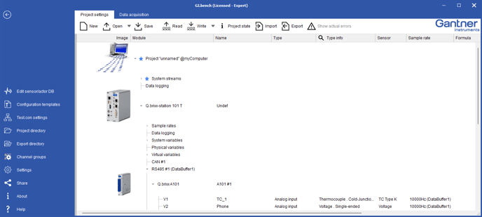
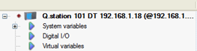
- The controller and connected measurement modules are shown in the project.
Configuring a Controller
Controller’s Sample Rate (Q.station)
- Double-click on the controller to open the Controller Settings window. In the Synchronization section you can modify the main sample rate
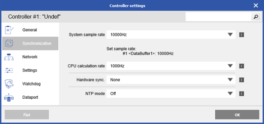
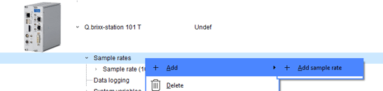
- Additional sample rates (up to 4 in a Q.station) can be added by right-clicking the Sample Rate section beneath the Q.station
- Double-click the created sample rate to modify. The name, sample frequency, and buffer size of each sample rate can be set. The sample frequency can be set as high as 100 kHz. The 1st sample rate is the master rate. The 2nd, 3rd, and 4th sample rate can be the same or less as the 1st sample rate.
The buffer size of each sample rate can be modified. There is 200 MB of data buffer space that can be split among the 4 x optional buffers.
The 1st sample rate receives its synchronization from the internal time clock. The 2nd, 3rd, or 4th sample rates can receive their synchronization from the internal time clock or one of the built-in digital inputs of a Q.station.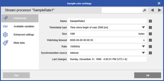
- The 1st sample rate receives its synchronization from the internal time clock. The 2nd, 3rd, or 4th sample rates can receive their synchronization from the internal time clock or one of the built-in digital inputs of a Q.station.
PAC Functionality Activation/Deactivation
- There are many functional possibilities with the built-in PAC functionality of a Gantner test controller. To program the PAC functionality within a controller, we need the test.con software. To create and download a test.con project to a controller the controller needs to be a “T” version. This must be specified at the time or purchase. This functionality must be activated.
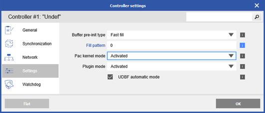
- In the controller settings, navigate to Settings section and change the Pac kernel mode
- More info on creating and downloading a test.con program into a Gantner test controller can be found on our test.con site or this intro article
UART Configuration
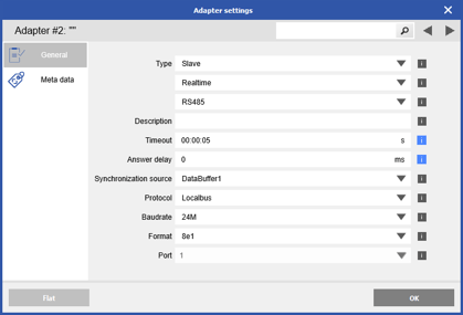
It is possible to configure the UARTs on a controller (4 x on Q.station). These settings can be found by double-clicking on respective RS485 section.
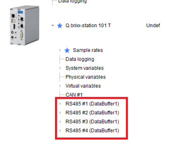
The most important setting to consider is baud rate, which can be configured up to 24M (48M on a Q.station X). When the sample rate of the controller is reduced, it might be necessary to reduce the baud rate also.
Life Signal (Q.station only)
The Q.station has built-in digital I/O, which can be used as life signals for various conditions.
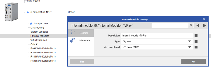
- The switching threshold for the digital inputs can be set for TTL or HTL. Double-click on the Physical variables section and modify the dig. input level parameter.
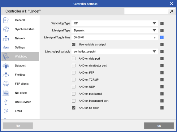
- A channel with an output direction on a Q.station can be used as a life signal based on preset conditions. The conditions can be switched on/off and can be combined as either AND/OR logic. To modify these settings, double-click on the Q.station and navigate to the Watchdog section
Interfaces (Q.station)
The Q.station has various communications interfaces for data transfer and data storage. These interfaces include CAN, EtherCAT, FTP, network drives, and E-mail. Configuring these interfaces can be found by double-clicking on the Q.station and navigating to corresponding section:
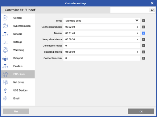
More information about how to utilize and apply these interfaces can be found on separate start-up guides in the Gantner knowledgebase.
Synchronization Source
The controller can obtain its synchronization internally (built-in real time clock) or externally (via SNTP, IRIG, GPS, AFNOR, or another Q.series controller). Double-click on the controller and navigate toSynchronization > Hardware sync. If set to “none” the controller obtains its synch internally. Select a different method using the drop down menu.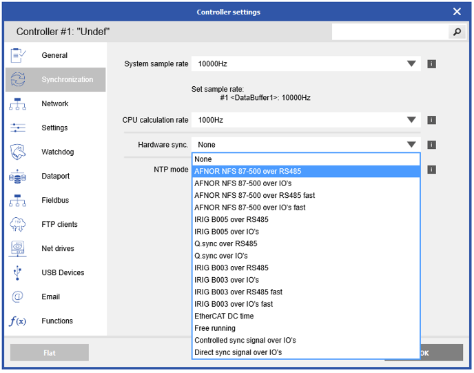
To synchronize the controller via SNTP change the NTP mode double-click on the controller and navigate to Host Interface > SNTP > Client Settings. Change the SNTP mode from Off to On. Enter the IP address of the location of the SNTP server. More information can be found in the “Synchronization via SNTP” guide on the Gantner website: LINK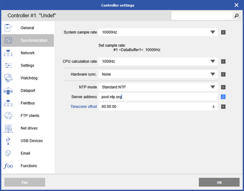
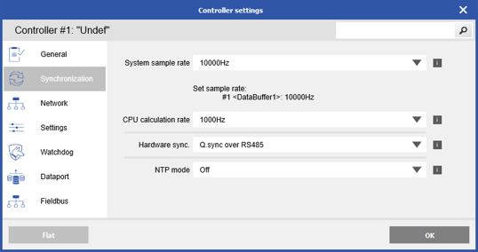
To synchronize the controller to another controller, set the Input Synchronization Protocol to Q.sync over RS485. Please see the “Synchronization of Multiple Controllers” guide on the Gantner website for more details: LINK
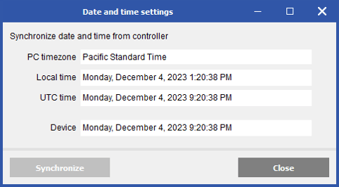
If the Input Synchronization Protocol is set to “none”, then we can perform a one-time synch of the controller’s internal clock with UTC-0 time. GI.bench then handles the offset based on the PC's timezone.
- Right-click on the Q.station > Set RTC
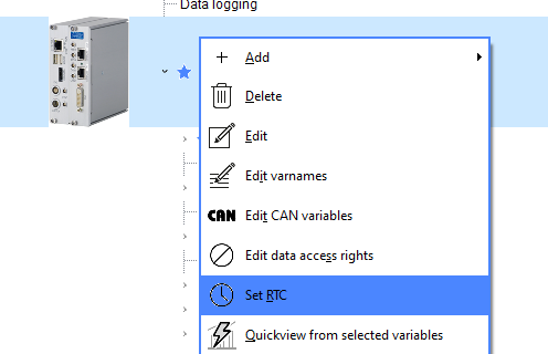
- Click Synchronize
Channel Configuration
Real Variables
A real variable is configured by double-clicking the channel in the project window
- Double-click on channel to configure. You can select multiple channels also > right-click > Edit
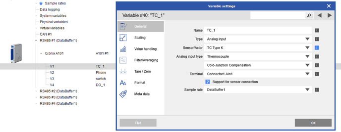
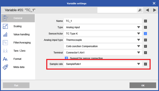
- General: change name, signal type, sensor type, analog input type, terminal, sample rate. New input types can be added to the sensor database to be selected form here.
https://knowledge.gantner-instruments.com/building-custom-sensor-tables - Scaling: change units, scaling method. Can scale by Factor and Offset, 2 point calculator, or 2 point measurement
https://knowledge.gantner-instruments.com/channel-scaling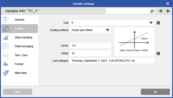
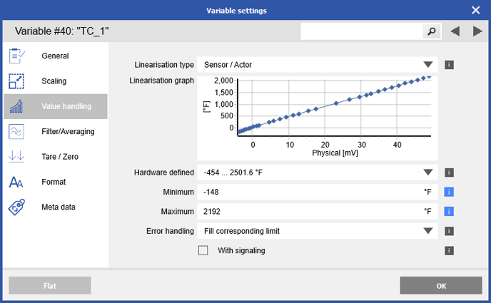
- Value Handling: change linearization type (sensor/polynomial), measurement range (some modules have multiple input ranges), min/max, and error handling behavior (how channel behaves on sensor disconnect)
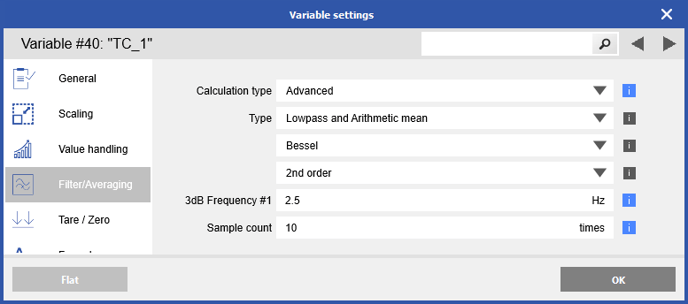
- Filter/Averaging: Configure module level filters and/or averaging. Can have standard (averaging, low pass, high pass, band pass) plus advanced (Bessel or Butterworth) filters.
- Tare/Zero/Shunt: configure a tare, zero, or shunt (on specific strain gauge modules) manually (on host), or on another variable or digital input.
https://knowledge.gantner-instruments.com/zero-tare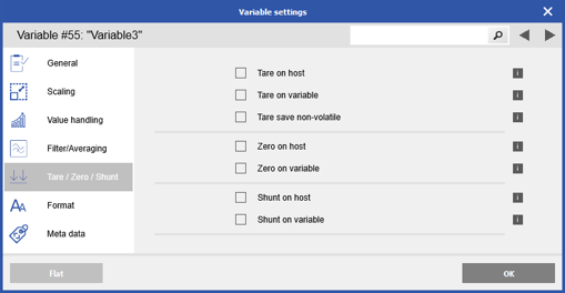
- Terminals: this column specifies which connector to use on the measurement module. Each Gantner measurement modules has 2 x connectors (a top and bottom). The top is connector 1 and the bottom is connector 2.

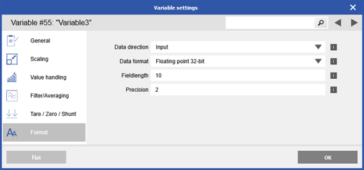
- Format: modify the way the variable is saved including the data direction, field length, precision, and format of the variable.
Virtual Variables
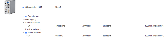
Virtual Variables are variables that are composed of real variables and/or other virtual variables. These variables can be created inside the measurement module in the form of arithmetic channels, signal conditioning channels, or set points. They can also be created inside the controller under the virtual variables section.
Inside the Measurement Module
- Right-click the module > Add > Add
- Double-click the newly created variable. In General > Type, select from Setpoint, Arithmetic, or Alarm
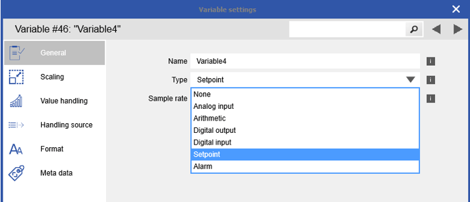
- Arithmetic – uses standard math functions such as adding, subtracting, multiplying, and dividing. Also available are min, max, rms, and integration. Real and other virtual variables within the same measurement module can be used. Arithmetic variables are not computed at the same speed as the real variables.
- Signal Conditioning – similar to the arithmetic channels but doesn’t have the ability to perform addition, subtraction, multiplication, and division. These variables are calculated at the same speed as the other real variables.
- Setpoint – the value of the set point can be obtained within the same module (source: internal) or from another measurement module (source: external). It can also be set to a constant.
- Alarm – outputs a 0 if none of the conditions are met, otherwise it outputs a 1. Each alarm can have up to 4 x separate conditions that are combined as logical OR. The conditions to select from are shown below:

- Arithmetic – uses standard math functions such as adding, subtracting, multiplying, and dividing. Also available are min, max, rms, and integration. Real and other virtual variables within the same measurement module can be used. Arithmetic variables are not computed at the same speed as the real variables.
Inside the Test Controller
- The Virtual Variables section is available under the test controller. Right-click on this section > Add > Add
- Select the type of virtual variable to add from the list shown above. It will be added to the virtual variables section.
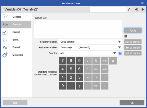
- Arithmetic – this is the most general version that can be used with the most flexibility. Standard math functions are available (adding, subtracting, multiplying, and division) along with a library of functions (i.e. average, min/max, comparison, PID). Any variable (real or virtual) within the same controller can be used within the arithmetic.
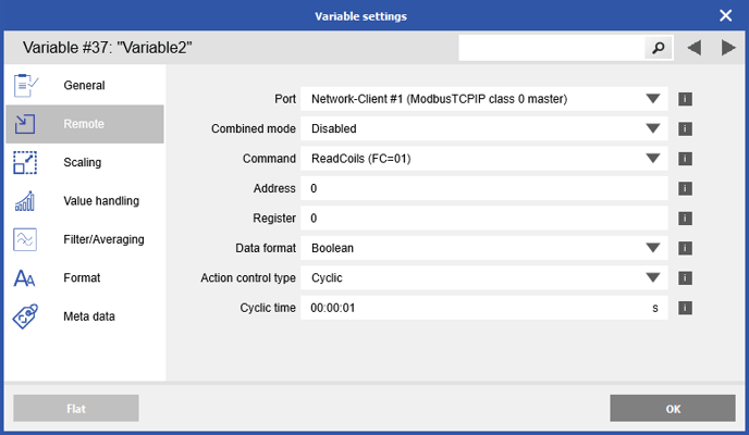
- Remote: can be set to Modbus, CAN, or Stream Processor
- Modbus – slave devices can interface directly with a Q.station via TCP over the Ethernet connection or via RTU over the USB port. These have to first be configured in the controller settings (TCP: Network > Client count > Type, RTU: USB Devices > Device count > Device type) For Modbus RTU connect an RS232 to RS485 converter (i.e. ISK103) between the Q.station and the slave. Configure the Modbus variable with the correct register settings/format.
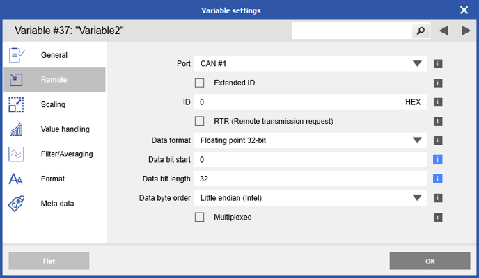
- CAN Input – it is possible to read and write CAN data with the Q.station. We setup the CAN inputs under the virtual variables section. Double-click on the CAN Input to modify the CAN ID, byte order, format, start bit, and bit length. If a CAN data base file is available, the pre-defined variables can be selected from this file.
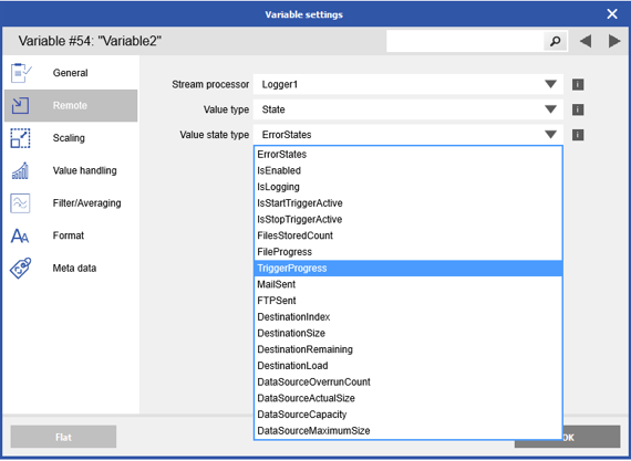
- Stream Processor - Create variables to monitor or control a data logger defined in the Q.station
- Modbus – slave devices can interface directly with a Q.station via TCP over the Ethernet connection or via RTU over the USB port. These have to first be configured in the controller settings (TCP: Network > Client count > Type, RTU: USB Devices > Device count > Device type) For Modbus RTU connect an RS232 to RS485 converter (i.e. ISK103) between the Q.station and the slave. Configure the Modbus variable with the correct register settings/format.
- Set point – a standard set point can be created here. The format of the variable is also available.
- Arithmetic – this is the most general version that can be used with the most flexibility. Standard math functions are available (adding, subtracting, multiplying, and division) along with a library of functions (i.e. average, min/max, comparison, PID). Any variable (real or virtual) within the same controller can be used within the arithmetic.
Naming Variables in Batches
Naming a variable (real or virtual) is as easy as typing in the desired name. This method is perfect for small to medium sized projects. When large projects are being created it might be necessary to name variables in batches, especially for identical sensors that are simply incrementing (Volts 1, Volts 2, …, Volts 20, etc.).
- In GI.bench, right-click anywhere and select Edit Varnames. You can also select multiple variables already > right-click > Edit varnames.
- In the Edit variable names window, select one or more variables to edit. Select from the available shortcuts to modify the naming rule-string. Apply to only selected or all.
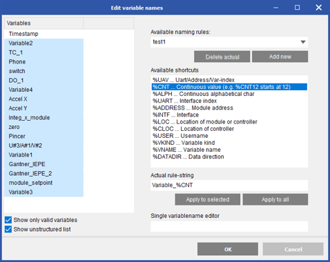
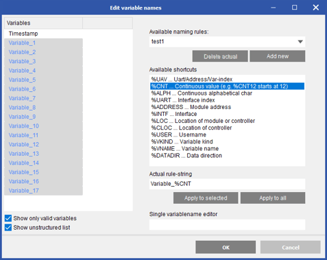
- Change single channel names by highlighting the channel and editing the Single variablename editor section
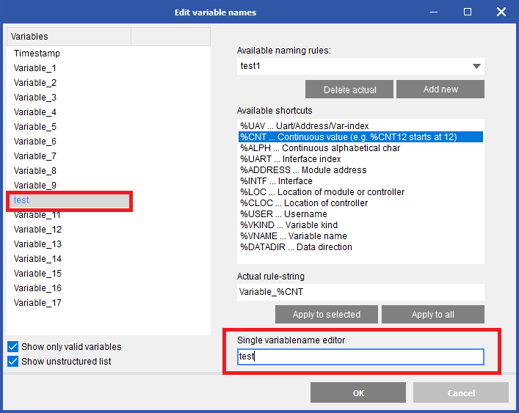
- Click OK to save changes
Data Logger Configuration – Q.station
See this article for more information on configuring a Q.station data logger: https://knowledge.gantner-instruments.com/q.station-data-logger-guide-gi.bench
Sample Rate Assignment
- Configure the number of data buffers to create by adding as many sample rates as needed by right-clicking the sample rate section > Add > Add sample rate
- For each sample rate, give it a name, sample frequency, and buffer size.
The name is used to distinguish one sample rate from the rest.
The sample frequency is the update rate of the buffer. This can be configured up to 100 kHz.
The buffer defines how large the buffer is. There is 200 MB available that must be shared between all buffers (up to 4).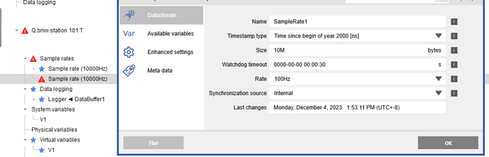
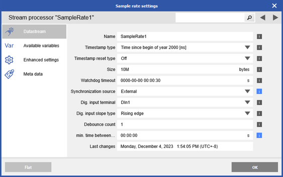
- As mentioned previously, the 1st sample rate obtains its synchronization internally. The synchronization source for sample rates 2 to 4 can be obtain internally or externally. To set externally, change the synchronization source:
- Additional settings become available when set to external.
Apply Sample Rate to Measurement Modules
There is a Sample rate column in the GI.bench project settings window. Edit the variable(s) as needed by right-clicking > Edit. Select the desired sample rate
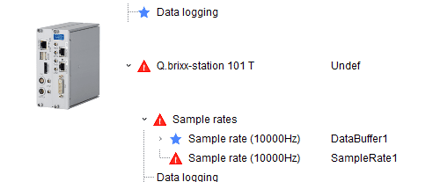
The measurement modules in the GI.bench project are listed under the UART/RS485 line they are configured to and sorted numerically by descending address.
Project Verification
System Check
GI.bench checks as the system is configured. Any errors or warnings must be fixed before updating the project to the controller. Right-click any section with an Error > More info to get more details
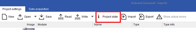
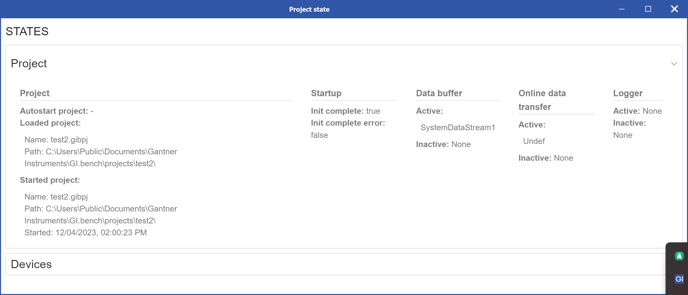
Once configuration is done, you can check the project and device state by select the Project state icon in the toolbar
Acquistion will be prompted to start to check in real time if there is any errors present. Error states will be shown at the bottom and any communication issues will on the UARTs will be shown next to the corresponding UART as an error count
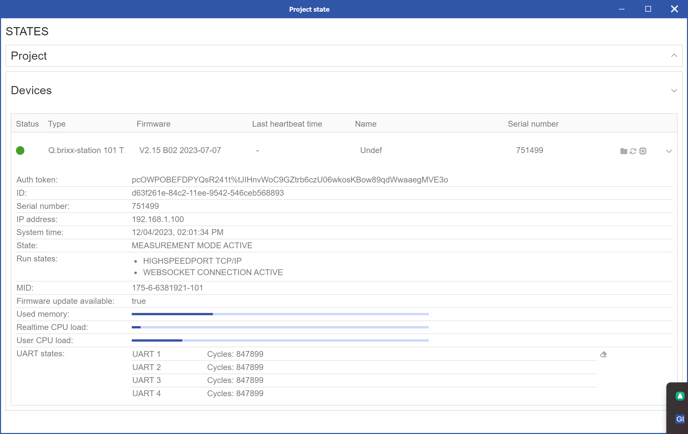
More info on the project can be seen by expanding the Project section
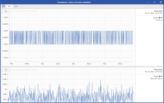
Viewing & Saving Live Data
After the project has been verified and updated to the controller it is now possible to view the live data stream. Switch to the Data Acquisition tab.
Data Acquisition will start as shown in the toolbar status
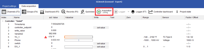
Channels: view all channels that are part of the FPGA. Can also set values, tares, zero, shunts.
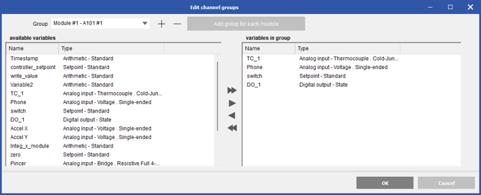
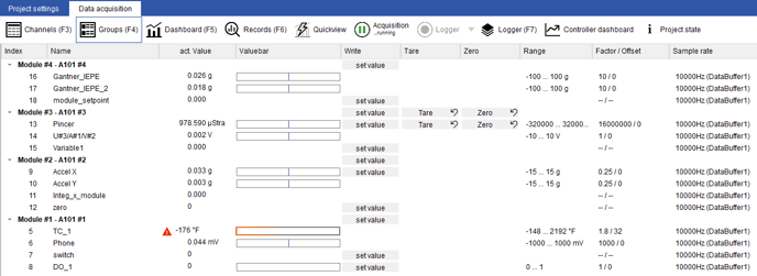
Groups: view channels in groups defined in the left-side channel group settings
Click on either Dashboard (project) or Controller Dashboard (controller) to configure the visualization dashboards.
Exporting Projects
The GI.bench project is saved in the projects folder within the Gantner directory of the PC (default: C:\Users\Public\Documents\Gantner Instruments\GI.bench\projects). When the project is updated to the controller, it is also saved inside the controller.
To modify the project on a different PC:
- Install GI.bench and run
- Connect the hardware to the new PC using a standard Ethernet cable.
- Open GI.bench and read
- Select Q.station and click OK.
- The project that had been inside the controller is now available on the new PC.
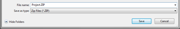
It is also possible to take a project that is open in GI.bench and export it to a ZIP file. This ZIP file can then be transferred to a different PC using an external storage device (i.e. USB thumb drive).
- Export > Project ZIP Archive. Click OK.
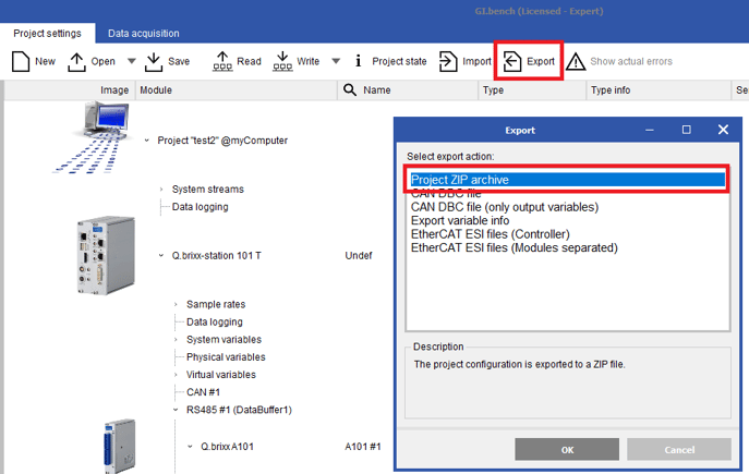
- Give the ZIP file a name and click Save.
Configuration (test.commander)
Applying the License & New Project
- After download and installing test.commander, start the program by clicking on the test.commander icon.
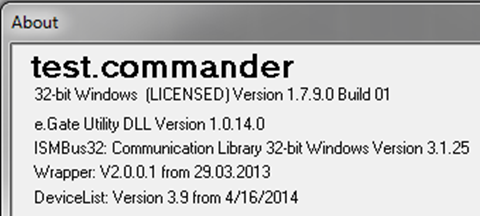
- Opening test.commander on a new PC for the first time will open in DEMO mode. Entering a test.commander license will convert the program into LICENSED mode. Enter the license information into the window provided:
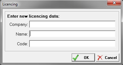
- When the license is entered successfully, the program will change to licensed mode.
- commander is now ready to create a new project.
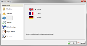
- Language settings may need to be set. Extras > Settings, navigate to Language:
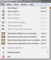
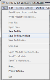
- Select File > New Project.
- Give the project a name.
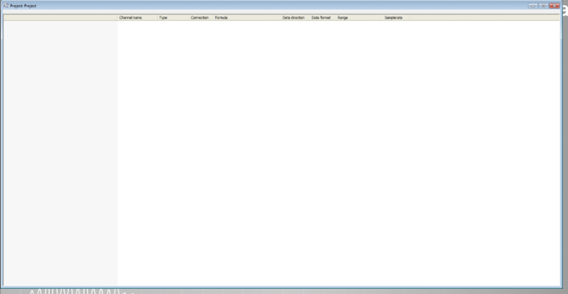
- A blank project is now available.
Slave Setup
- When a new system is being used, the first step is to assign a unique address to each measurement I/O module. There are two ways to assign an address to a measurement module: via the DIP switches mentioned in the previous assembly section or using test.commander. In this section, we will discuss how to set the address using the software method.
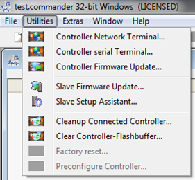
- With a blank project open, select Utilities > Slave Setup Assistant:
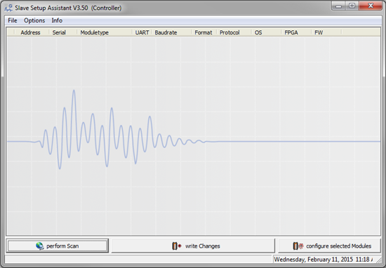
- The Slave Setup Assistant window will appear. Click on the perform Scan button to search for the attached controller.
- A separate window appears with all connected controllers. Highlight the controller for the current system and click OK.
- The program will scan all UARTs (2 on a Q.gate and 4 on a Q.station/Q.pac) to search for all connected measurement modules. All modules that are found will be displayed in the Slave Setup Assistant window:
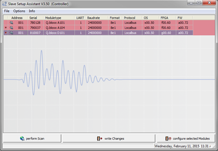
- All measurement modules are shipped from the factory with a default address of 1. To modify the address of any module, click in the cell under the Address column to change the address. Repeat the process for all modules.
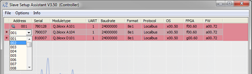
- Click the write Changes button to apply the new settings.

Firmware Updates
- New Gantner hardware (controllers and measurement modules) are shipped from the factory with the most up to date version of the firmware loaded. However, it is good practice to verify if the system has the most current firmware version from time to time. New firmware versions for controllers and measurement modules are included when a new version of test.commander is installed.
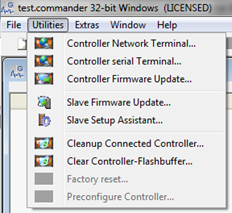
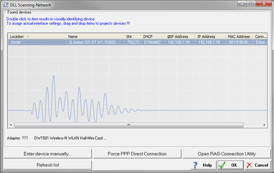
- To check the firmware of a controller, select Utilities > Controller Firmware Update:
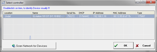
- The program will search for all connected controllers, highlight the controller to connect to and click the OK button.
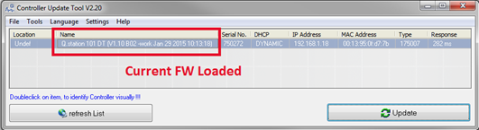
- The Controller Update Tool appears, highlight the controller to update and click the Update button.
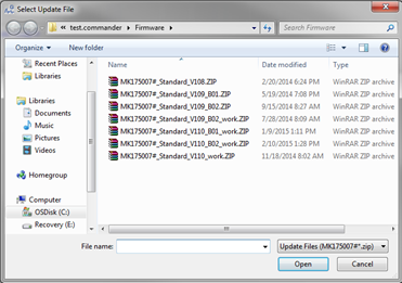
- A window will appear with all FW versions available on the current PC. Select the FW to update the controller with and click the Open button. If the controller already has the most up to date version, an update is not required.
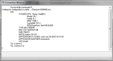
- For a controller that requires an update, an FTP Connection Window will display the update process. DO NOT remove power to the controller and DO NOT disconnect the Ethernet cable during the update process.
- To check the firmware version of a measurement module, select Utilities > Slave Firmware Update:

- The Slave Firmware Update window appears, click the perform Scan button.

- Highlight the controller to connect to and click the OK button.
- The software scans all the modules. A green check mark represents an up to date module and a red mark means the module needs to be updated.
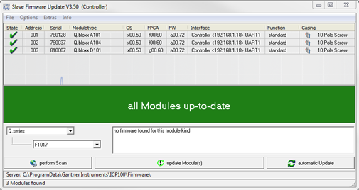
- Clicking on the update Module(s) button will update all modules that require an update.
Connecting to the Hardware
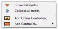
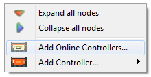
- Within the blank project, right-click on the mouse and select Add Online Controllers.
- Select the controller to add to the project and click the OK button.
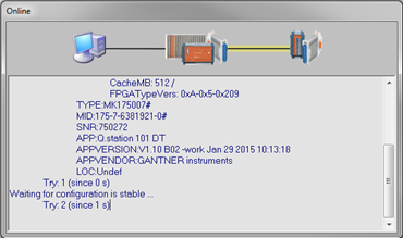
- The Online window displays the read process of the controller.
- The following window appears at the end of the process, click OK.
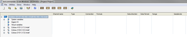
- The controller and connected measurement modules are shown in the project.
Configuring a Controller
Controller’s Sample Rate (Q.station)
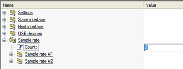
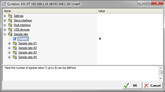
- Double-click on the controller and navigate to Sample rate.
- It is possible to have up to 4 x different sample rates in a Q.station. Change the count value to add more samples rates.
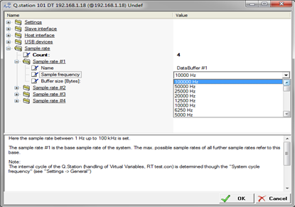
- The name, sample frequency, and buffer size of each sample rate can be set. The sample frequency can be set as high as 100 kHz. The 1st sample rate is the master rate. The 2nd, 3rd, and 4th sample rate can be the same or less as the 1st sample rate.
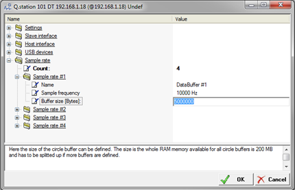
- The buffer size of each sample rate can be modified. There is 200 MB of data buffer space that can be split among the 4 x optional buffers.
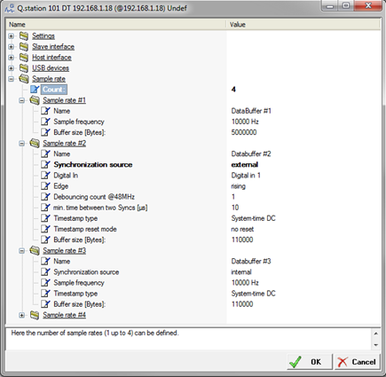
- The 1st sample rate receives its synchronization from the internal time clock. The 2nd, 3rd, or 4th sample rates can receive their synchronization from the internal time clock or one of the built-in digital inputs of a Q.station.
Controller’s Sample Rate (Q.gate)
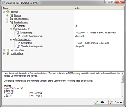
- Double-click on the controller and navigate to Settings > Databuffer gen. It is possible to have 1 or 2 data buffers in a single Q.gate. Both buffers use the same sample rate, but each buffer’s size can be modified. There is 16 MB available between all buffers.
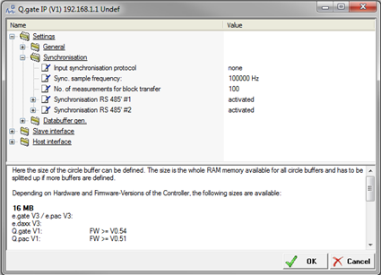
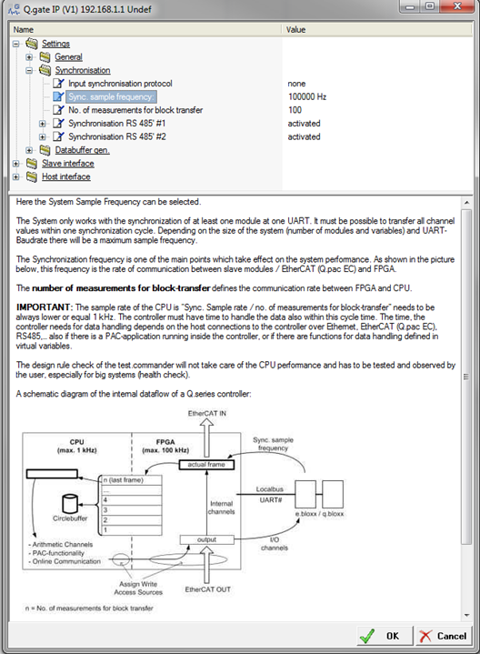
- Navigate to Settings > Synchronization. The Sync. sample frequency can be modified:
- When the Sync. sample frequency is modified, the No. of measurements for block transfer also needs to be modified. The number of measurements for block transfer defines the communication rate between the FPGA and CPU. The rule to follow is:
PAC Functionality Activation/Deactivation
- There are many functional possibilities with the built-in PAC functionality of a Gantner test controller. To program the PAC functionality within a controller, we need the test.con software. To create and download a test.con project to a controller the controller needs to be a “T” version. This must be specified at the time or purchase. This functionality must be activated.
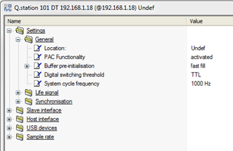
- In a Q.station, navigate to Settings > General > PAC Functionality to activate or deactivate the feature.
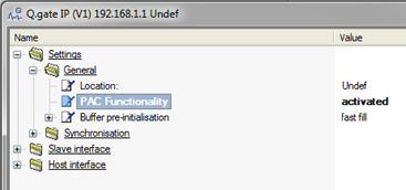
- In a Q.gate, navigate to Settings > General > PAC Functionality to activate or deactivate the feature. When the PAC functionality is activated in the Q.gate, the data buffer can no longer be modified. The test.con program is saved to this memory.
- Creating and downloading a test.con program into a Gantner test controller will be explained in further detail in a separate document.
test.con with Q.station: LINK
test.con with Q.gate: LINK
UART Configuration
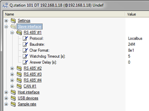
It is possible to configure the UARTs on a controller (2 x on Q.gate and 4 x on Q.station/Q.pac). These settings can be found by double-clicking on the controller and navigating to Slave interface. The most important setting to consider is baud rate, which can be configured up to 24M. When the sample rate of the controller is reduced, it might be necessary to reduce the baud rate also.
Q.station:
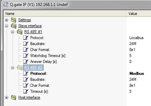
Q.gate:

The 2nd UART of a Q.gate can be configured to use the Modbus protocol.
Life Signal (Q.station only)
The Q.station has built-in digital I/O, which can be used as life signals for various conditions.
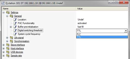
- The switching threshold for the digital inputs can be set for TTL (5V) or PLC (10V) levels. Double-click on the Q.station and navigate to Settings > General > Digital switching threshold to modify this setting. This applies for all inputs.
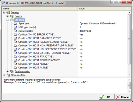
- The digital outputs on a Q.station can be used as a life signal based on preset conditions. The conditions can be switched on/off and can be combined as either AND/OR logic. To modify these settings, double-click on the Q.station and navigate to Settings > Life signal.
Interfaces (Q.station)
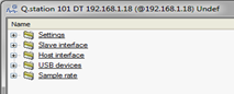
The Q.station has various communications interfaces for data transfer and data storage. These interfaces include CAN, EtherCAT, FTP, network drives, and E-mail. Configuring these interfaces can be found by double-clicking on the Q.station and navigating to Host interface:
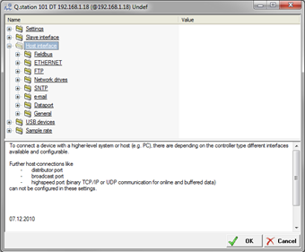
More information about how to utilize and apply these interfaces can be found on separate start-up guides on the Gantner website: LINK
Synchronization Source
The controller can obtain its synchronization internally (built-in real time clock) or externally (via SNTP, IRIG, GPS, AFNOR, or another Q.series controller). Double-click on the controller and navigate to Settings > Synchronization > Input Synchronization Protocol. If set to “none” the controller obtains its synch internally. Select a different method using the drop down menu.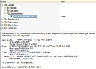
To synchronize the controller via SNTP double-click on the controller and navigate to Host Interface > SNTP > Client Settings. Change the SNTP mode from Off to On. Enter the IP address of the location of the SNTP server. More information can be found in the “Synchronization via SNTP” guide on the Gantner website: LINK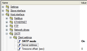
To synchronize the controller to another controller, set the Input Synchronization Protocol to Q.sync over RS485. Please see the “Synchronization of Multiple Controllers” guide on the Gantner website for more details: LINK
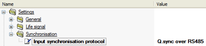
If the Input Synchronization Protocol is set to “none”, then we can perform a one-time synch of the controller’s internal clock with that of the attached PC.
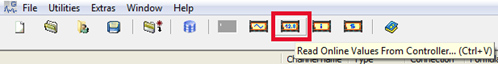
- Click on the Read Online Values From Controller button:
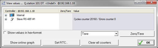
- Click on the Set RTC button:
- Make sure the radio button next to “Use local PC time” is selected. Click on the “Synchronize” button to apply the synch.
Time – date and time of the PC
Device – date and time of the controller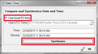
Channel Configuration
Real Variables
A real variable is configured in ICP100 (included with test.commander). Double-click on a module to open the module in ICP100. For this example, we will use an A101 module.
- Double-click on the A101 module to open the module in ICP100:
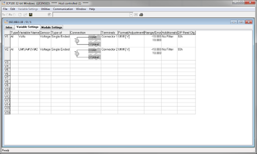
- A new module will have the default settings loaded. For example, an A101 is a 2 x channel universal input module. There are 16 x slots available in each module. If there are 2 x real variables used, there are 14 x remaining slots available for arithmetics, signal conditioning, set points, and alarms.
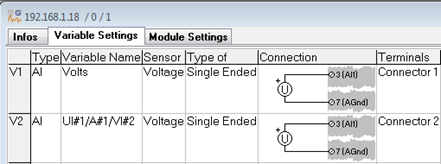
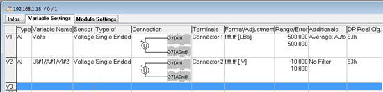
- Type: this column selects the type of variable (varies by module type). A real variable is an AI (Analog Input), AO (Analog Output), DI (Digital Input), or DO (Digital Output).
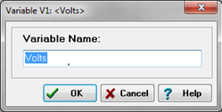
- Variable Name: this column is used to give the variable a custom name. Each variable within a single controller needs to have a unique name.
- Sensor: this column specifies the type of variable. The type of sensor to choose depends on the type of module being used. An A101 module is a universal input module, therefore many possibilities are available:
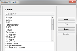
A modified version of any sensor can be created. This is necessary for sensors that have very precise calibration points. For example, a thermocouple can be factory calibrated.
Highlight the sensor to modify and click on the Copy button.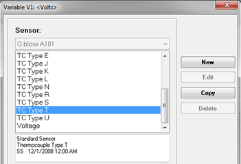
Give the new sensor a name.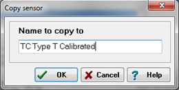
The new sensor will be added to the list. Highlight the new sensor and click on the Edit button.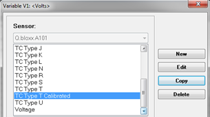
The sensor configuration window appears. This window provides more information about the pre-configured sensor. Click on the Lineariz. button.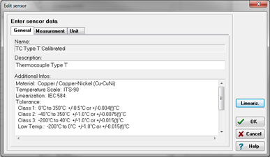
Highlight the unit to modify and click OK.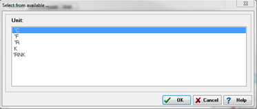
A sensor linearization table will appear. There are 300 individual measurement points that can be used. Enter the measured value and displayed value for each point. The table can be exported and modified in a spreadsheet by clicking the Export button. A modified table can be imported by clicking on the Import button.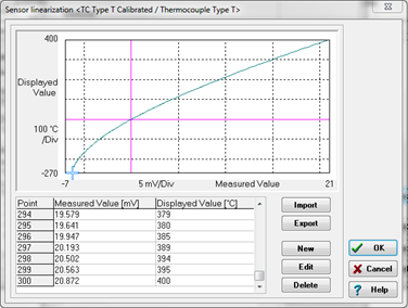
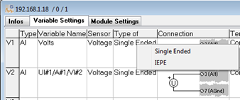
Click OK to apply the new settings. - Type of: this column specifies the type of sensor (varies by module and by sensor). For example, if a Voltage sensor is used on an A101, it can be configured as a single ended or IEPE sensor.
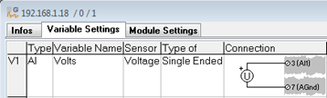
- Connection: this column displays which PINs the sensor is physically connected to. In the example below, the voltage sensor is wired across PINs 3 and 7.
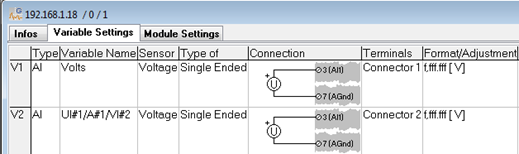
- Terminals: this column specifies which connector to use on the measurement module. Each Gantner measurement modules has 2 x connectors (a top and bottom). The top is connector 1 and the bottom is connector 2.
- Format/Adjustment: this column is used to modify the way the variable is saved including the units and format of the variable.
The variable can use the pre-defined unit selected based on the type of sensor used (for example, voltage sensor uses V or mV). However, the variable can be scaled to engineering units. Enter the units to use and click on the Scaling button.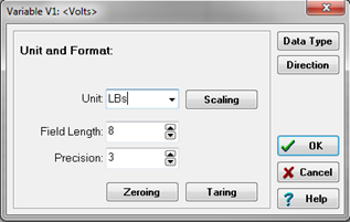
The variable can be scaled using either of 2 x methods: point-point calibration or factory/offset. For this example we will use the point-point calibration method.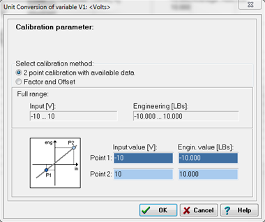
There are 2 x columns, the input value and the Engin. value. There are 2 x points for each column, a low end and high end. The input value represents the physical characteristic that the sensor is measuring (i.e. Volts). The Engin. value represents the measured quantity that we wish to save (i.e. LBs).
For this example, a ±10V input could represent ±500 LBs: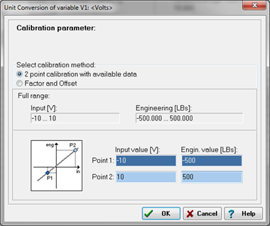
Click OK to confirm the setting changes.
Calibrating channels using live values: LINK
The Field Length sets the maximum number of digits the sensor will display.
The Precision sets the number of decimal places.
The Field Length needs to be at least 2+ the Precision.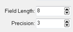
Zeroing and Taring are also configured in this section. A separate quick start guide that discusses how to apply the zero and tare feature can be found on the Gantner Instruments website: LINK - Range/Error: this column sets the minimum and maximum value to display. A value not within this range will result in an error/sensor failure. The behavior at sensor failure is also configured in this section. At failure, the sensor will display either:
- Corresponding Limit
- Stay at Last Value
- User selected Default Value
This error handling can be activated or deactivated.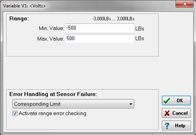
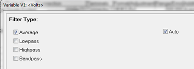
- Additionals: this column adds/removes/modifies any filters (average, lowpass, highpass, or bandpass).
Virtual Variables
Virtual Variables are variables that are composed of real variables and/or other virtual variables. These variables can be created inside the measurement module in the form of arithmetic channels, signal conditioning channels, or set points. They can also be created inside the controller under the virtual variables section.
Inside the Measurement Module
- Double-click on the measurement module to open it in ICP100.
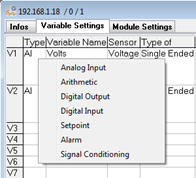
- Find the next empty variable (V3 below) and click inside the Type column.
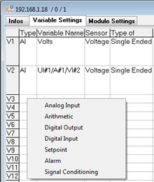
- Select the type of virtual variable to create:
Arithmetic – uses standard math functions such as adding, subtracting, multiplying, and dividing. Also available are min, max, rms, and integration. Real and other virtual variables within the same measurement module can be used. Arithmetic variables are not computed at the same speed as the real variables.
Set point – the value of the set point can be obtained within the same module (source: internal) or from another measurement module (source: external). It can also be set to a constant.
Alarm – outputs a 0 if none of the conditions are met, otherwise it outputs a 1. Each alarm can have up to 4 x separate conditions that are combined as logical OR. The conditions to select from are shown below: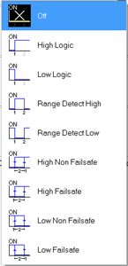
Signal Conditioning – similar to the arithmetic channels but doesn’t have the ability to perform addition, subtraction, multiplication, and division. These variables are calculated at the same speed as the other real variables. - After selecting the type of variable, the specifics of the variable can be modified under the Additionals column. For example, the formula for an arithmetic variable can be created.
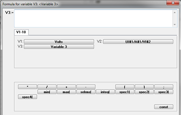
- Make sure to save the configuration before closing ICP100.
Inside the Test Controller
- The Virtual Variables section is available under the test controller. Right-click on this section to add a new variable.
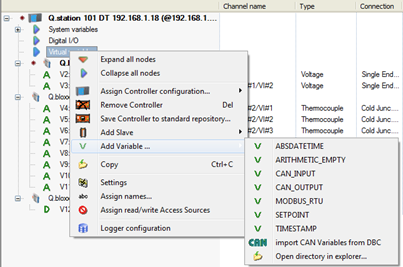
- Select the type of virtual variable to add from the list shown above. It will be added to the virtual variables section.
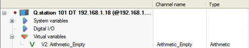
Arithmetic Empty – this is the most general version that can be used with the most flexibility. Standard math functions are available (adding, subtracting, multiplying, and division) along with a library of functions (i.e. average, min/max, comparison, PID). Any variable (real or virtual) within the same controller can be used within the arithmetic.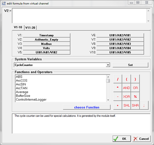
Modbus – slave devices can interface directly with a Q.station via the USB port. Connect an RS232 to RS485 converter (i.e. ISK103) between the Q.station and the slave. Configure the Modbus variable with the correct register settings/format.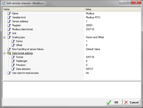
CAN Input – it is possible to read and write CAN data with the Q.station. We setup the CAN inputs under the virtual variables section. Double-click on the CAN Input to modify the CAN ID, byte order, format, start bit, and bit length. If a CAN data base file is available, the pre-defined variables can be selected from this file; click the CAN DB button to navigate to the file.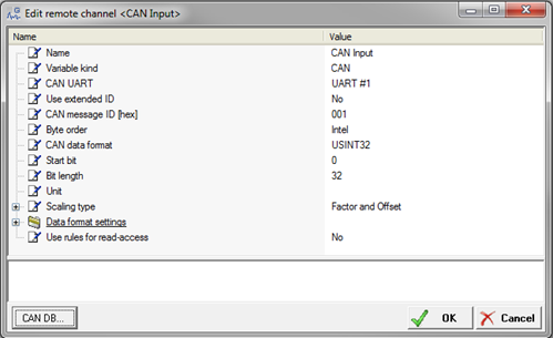
Set point – a standard set point can be created here. The format of the variable is also available.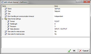
Naming Variables in Batches
Naming a variable (real or virtual) is as easy as typing in the desired name. This method is perfect for small to medium sized projects. When large projects are being created it might be necessary to name variables in batches, especially for identical sensors that are simply incrementing (Volts 1, Volts 2, …, Volts 20, etc.).
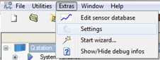
- In test.commander, select Extras > Settings.
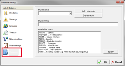
- Select the Variable Names option.
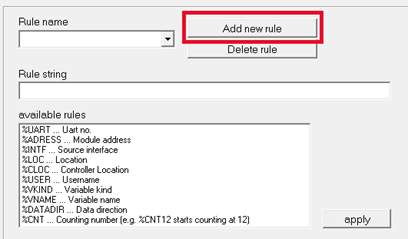
- Click on the Add new rule button.
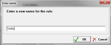
- Give the rule a name.
- Define the variable’s format in the Rule string section.
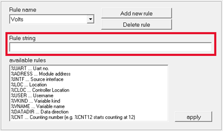
- Use the pre-set rules to create the custom string. For example:
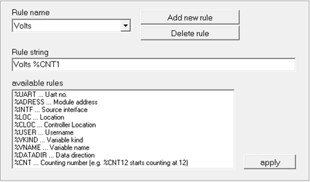
- Click the OK button to save the rule.
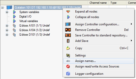
- Right-click on the controller and select Assign names.
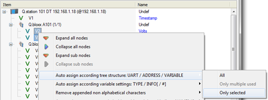
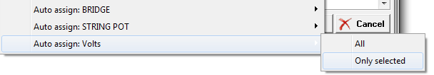
- Highlight the Variables to rename and right-click on the selected variables.
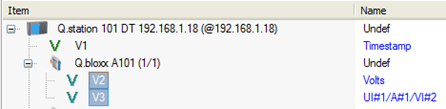
- It is possible to auto assign names using the pre-set methods (UART/ADDRESS/VARIABLE or TYPE/INFO) or using one of the rules we created.
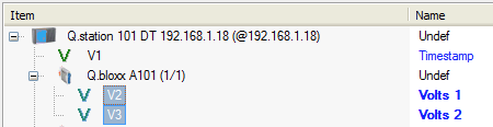
- Click the OK button to apply the new settings. The variables have been renamed in the project, make sure to update the project to the controller to finalize the process.
Data Logger Configuration – Q.station
This section describes how to configure the Q.station’s data logger. For complete information, please use this guide along with the Q.station manual (page 59-85).
Rules
The data logger built into the Q.station is very flexible but there are some rules to follow in order to create a functional system.
- It is possible to configure up to 4 x separate data buffers. Each data buffer can have a unique sample rate. The 1st data buffer is the master rate; the 2nd, 3rd, and 4th buffers can be configured to have the same sample rate or smaller (can’t be greater than the 1st)
- It is possible to configure up to 4 x separate UARTs on a single Q.station. A single UART can be configured for 1 x data buffer (i.e. 1 x sample rate). Modules/channels under a single UART can’t be split into more than 1 x data buffer.
Incorrect: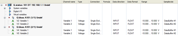
Correct: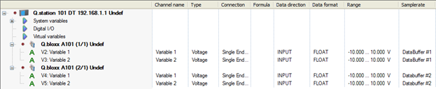
- The 1st data buffer is the basic sample rate of the entire Q.station, therefore it must obtain its synchronization source internally. Data buffers 2 to 4 can obtain its synchronization internally or externally (i.e. angular synchronization).
- It is possible to create up to 20 x separate data loggers within a single Q.station.
- A single data logger can obtain data (i.e. channels/variables) from 1 x data buffer.
- The logging rate of a data logger can be the same or less than the data buffer it is assigned to.
Sample Rate Assignment
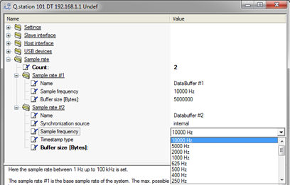
- Configure the number of data buffers to create. Double-click on the Q.station and navigate to Sample rate > Count. Enter the number of sample rates (1 to 4).

- For each sample rate, give it a name, sample frequency, and buffer size.
The name is used to distinguish one sample rate from the rest.
The sample frequency is the update rate of the buffer. This can be configured up to 100 kHz.
The buffer defines how large the buffer is. There is 200 MB available that must be shared between all buffers (up to 4).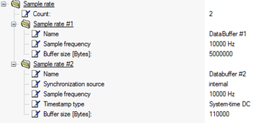
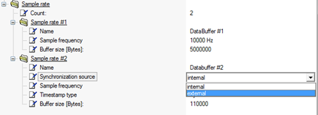
- As mentioned in the rules section, the 1st sample rate obtains its synchronization internally. The synchronization source for sample rates 2 to 4 can be obtain internally or externally. To set externally, change the synchronization source:
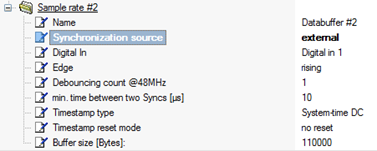
- Additional settings become available when set to external. Please see pages 60-61 and 85 of the Q.station manual for more details: LINK
Apply Sample Rate to Measurement Modules
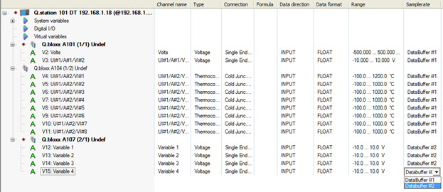
There is a Sample rate column in the test.commander project. Using this column, apply the desired sample rate for each channel. Remember that variables/channels located on a UART need to share the same sample rate.
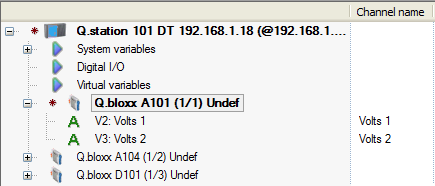
The measurement modules in the test.commander project display the UART and address for which they are configured.
Example:
Q.bloxx A101 (1/1) = Q.bloxx A101 (UART 1/Address 1)
Q.bloxx A104 (1/2) = Q.bloxx A101 (UART 1/Address 2)
Q.bloxx A107 (2/1) = Q.bloxx A101 (UART 2/Address 1)
Accessing Logger Configuration
The preliminary settings are now configured. Highlight the Q.station and click the Logger configuration button.
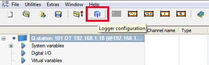
Complete details on how to configure the Q.station data logger: LINK
Data files saved using the Q.station data logger are saved as .DAT file format. These are universal data bin files (UDBF), a binary file that contains a header section followed by raw binary data. These .DAT files can be opened using test.viewer for post processing.
Project Verification
System Check
After configuring the controller, configuring all the channels/variables, and setting the data logger configuration, but before updating the project to the controller, it is beneficial to analyze the feasibility of the project.
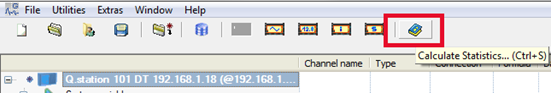
Select the Calculate Statistics button.
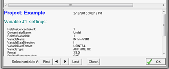
Select the Check button.
The Design Rule Check window will appear. The back ground color displays the feasibility:
White = Will work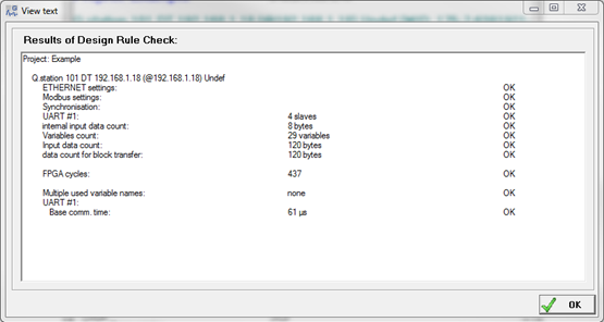
Red = Will not work
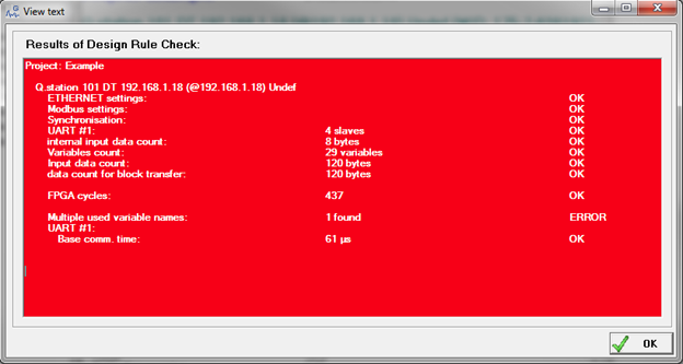
Yellow = Might work
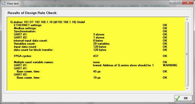
The cause of the issue is shown next to the warning/error. Change the appropriate settings before proceeding (sample rate, UART baud rate, number of channels, and variable names are just a few of the most common issues). After all settings have been correctly configured, the project can be updated back to the controller: File > Write Project (Update).
Viewing & Saving Live Data
After the project has been verified and updated to the controller it is now possible to view the live data stream. This is performed using the built-in tool called test.viewer.
Select the Read Online Values From Controller button:

The View Values window appears. Use this page to verify if all appropriate sensors are connected. Check if there are any data dropouts (if there are any error counters accruing).
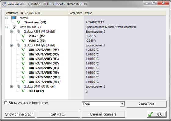
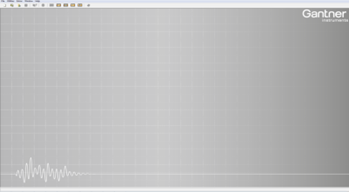
Click on the Show online graph button to open test.viewer.
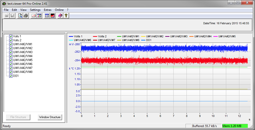
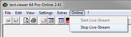
The data can be analyzed using test.viewer. To save the data, select Online > Stop Live Stream.
Select File > Save As.
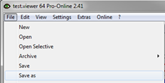
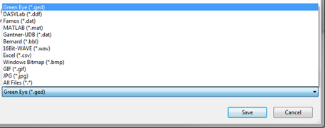
Select a name for the file and the format in which to save to.
Exporting Projects
The test.commander project is saved in the projects folder within the Gantner directory of the PC. When the project is updated to the controller, it is also saved inside the controller.
To modify the project on a different PC:
- Install test.commander and apply the license on the new PC.
- Connect the hardware to the new PC using a standard Ethernet cable.
- Open test.commander and create a new/blank project.
- Right-click in the work space and select Add Online Controllers.
- The project that had been inside the controller is now available on the new PC.
It is also possible to take a project that is open in test.commander and export it to a ZIP file. This ZIP file can then be transferred to a different PC using an external storage device (i.e. USB thumb drive) or E-mail.
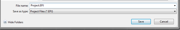
- File > Export Project
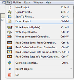
- Give the ZIP file a name and click Save.
Index
Q.bloxx Manual: http://www.gantnerinstruments.com/datasheets/manuals/gantner-q.bloxx-manual.pdf
Q.station Data Logger Configuration Guide: http://www.gantnerinstruments.com/datasheets/library/qstation-data-logger-guide.pdf
Q.station Email Configuration Guide: http://www.gantnerinstruments.com/datasheets/library/qstation-email-configuration-guide.pdf
Q.station FTP Configuration Guide: http://www.gantnerinstruments.com/datasheets/library/qstation-ftp-configuration-guide.pdf
Q.station Network Drives Configuration Guide: http://www.gantnerinstruments.com/datasheets/library/qstation-network-drives-configuration-guide.pdf
test.commander Licensing Information: http://www.gantnerinstruments.com/datasheets/library/test.commander-license.pdf
Point to Point Calibration with Live Values: http://www.gantnerinstruments.com/datasheets/library/point-to-point-calibration.pdf
Channel Configuration with ICP100: http://www.gantnerinstruments.com/datasheets/library/icp-100-channel-configuration.pdf
Zero/Tare Configuration: http://www.gantnerinstruments.com/datasheets/library/zero-tare-functionality.pdf
test.con Configuration with Q.gate: http://www.gantnerinstruments.com/datasheets/library/test.con-start-up-guide-qgate-qpac.pdf
test.con Configuration with Q.station: http://www.gantnerinstruments.com/datasheets/library/test.con-start-up-guide-qstation.pdf